Download
1 / 54
540 likes | 555 Views
Fluvial Hydraulics CH-3. Uniform Flow. Redefining Uniform Flow. Uniform flow if flow depth (h, D h ) as well as U, Q, roughness, and S f remain invariable in different cross sections Streamlines are rectilinear and parallel Vertical pressure distribution is hydrostatic

E N D
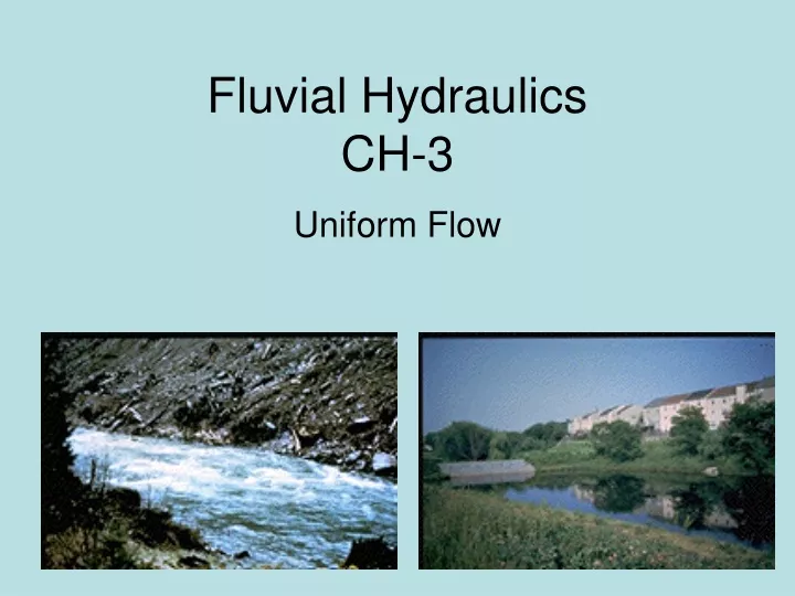
Fluvial HydraulicsCH-3 Uniform Flow
Redefining Uniform Flow • Uniform flow if flow depth (h, Dh) as well as U, Q, roughness, and Sf remain invariable in different cross sections • Streamlines are rectilinear and parallel • Vertical pressure distribution is hydrostatic • Flow depth under uniform flow called normal flow depth • Se = Sf = Sw
Redefining Uniform Flow • Uniform flow is rare in natural and artificial channels • Only possible in very long prismatic channels far distance from an upstream or downstream boundary conditions
Continuity Equation • From last time… • Let us also assume the flow is steady…
Equation of Motion • Start with prismatic channel… • Friction force acting on the wetted perimeter: • Longitudinal component of gravity force: • What do we know about these forces in uniform flow?
Equation of Motion • We can then obtain the expression… • In hydrodynamics, we usually define:
Equation of Motion • Sometimes you will see the use of a friction coefficient…
Equation of Motion • You can also write the Darcy-Weisbach equation as…
Different Friction (Resistance) Coefficients • Darcy-Weisbach (f) – data generally based on circular cross-sections and standard roughness values • Chezy Coefficient (C) – useful as long as the flow is turbulent • Manning’s (n) • Coefficient for Mobile Bed – estimation for an immobile bed is difficult and even more so for mobile bed
Friction Coefficient, f • Usually for pipes we use the Moody diagram or the relation of Colebrook-White for turbulent flow • For circular cross-sections, you can use the experiments performed on pipes, with the following modification:
Friction Coefficient, f • Colebrook-White (turbulent flow) – written for channels as… • See Table 3.1 for equivalent roughness (ks) for artificial channels • For granular beds, usually use ks = d50 • Suggestion by researchers to modify the hydraulic radius by a factor, f: • Rectangular (B = 2h) section f= 0.95 • Large Trapezoidal section f = 0.80 • Triangular (Equilateral) section f = 1.25
Friction Coefficient, f • For most channels, ks is large and flow is turbulent, so Re is large: • Rough, turbulent flow: What does this imply? • Justification for use of Chezy equation, where C is only a function of the relative roughness (ks /Rh)
Friction Coefficient, f • For turbulent, rough flow…
Friction Coefficient, f • If rough channels of large widths (Rh = h), f can be obtained from measurements of point velocities: • Graf derives this expression assuming logarithmic distribution (see data on next slide):
Friction Coefficient, f • Obtained from experimental measurements at two depths (z’=0.2h and z’=0.8h):
Chezy Coefficient, C • Only valid for turbulent, rough flow • Estimated using empirical methods based on the hydraulic radius (m, s): • Bazin formula – established with data from small artificial channels:
Chezy Coefficient, C • Kutter formula – established with data from artificial channels and larger rivers: • Forchheimer:
Chezy Coefficient, C • Manning’s Equation:
Manning’s Equation • Only valid for turbulent, rough flow • Actually Manning’s assumes a coefficient that stays constant for a given roughness • Chezy coefficient changes depending on the relative roughness (Rh) • Typically, n = 0.012-0.15 for natural and artificial channels
Discharge Calculations • Based on Manning’s equation… • Sometimes you will see the use of a term called the conveyance, K(h) – measure of the capacity for the channel to transport water:
Normal Depth • Solve Manning’s equation for h = hn… • Note that the normal depth can only exist on slopes that are decreasing (Sf>0)
Composite Sections • Can solve for case where different parts of the cross-section have different roughness or bed slope: • Apply formula of discharge for each subsection
Exercise 3.A - Graf A trapezoidal channel with bottom width of b = 5 m and side slopes of m = 3 is to built of medium-quality concrete to convey a discharge of Q = 80 m3/s. The channel slope is Sf = 0.1%. Flow is uniform at a temperature of 10oC. (a) Calculate the flow depth using both the Manning’s coefficient and the friction factor. (b) Verify whether the flow is laminar/turbulent and subcritical/supercritical.
Bed Forms – Mobile Bed • Mobile bed – channel composed on non-cohesive solid particles which are displaceable due to the action of flow • Bed deformations depending on flow: • Fr < 1 – Subcritical and two potential regimes: • No Transport and Flat Bedform: Velocity does not exceed the critical velocity for that sediment • Transport and Mini-dune or Dune: Growing lengths l
Bed Forms – Mobile Bed • Bed deformations depending on flow: • Fr = 1 – Critical: • Transport and Flat: Dunes which are already long are washed out and the bed appears to be flat (state of transition) • Fr>1 – Supercritical: • Transport and Anti-dunes: Dunes that travel in the upstream direction, water surface becomes wavy (impacted by dune)
Bed Forms – Mobile Bed • Geometry of dunes idealized as triangular by Graf
Bed Forms – Mobile Beds • Why are we concerned with bed forms? • They increase the resistance to flow… • Researchers have used superposition to analyze for the effects of roughness due to particles (t’) and roughness due to bed form (t’’):
Friction Coefficient – Mobile Beds • Two types of methods: • Direct Calculation: Determine the overall or entire f • Separate Calculation: Determine f’ using prior formulas and then f’’ using other formulas
Friction Coefficient – Mobile Beds • Direct Calculation (see textbooks for all formulas): • Sugio (1972): • KT = 54 (mini-dunes) • KT = 80 (dunes) • KT = 110 (upper regime) • KT = 43 (rivers with meanders) • Grishanin (1990):
Friction Coefficient – Mobile Beds • Separate Calculation (see textbooks for all formulas): • Einstein-Barbarossa: American Rivers (0.19<d35[mm]<4.3 and 1.49 x 10⁻⁴<Sf< 1.72 x 10⁻³)
Friction Coefficient – Mobile Beds • Alam-Kennedy: Artificial: 0.04<d50<0.54 (mm) Natural: 0.08<d50<0.45 (mm)
Discharge – Mobile Bed • Two velocities of concern with non-cohesive, mobile beds: • Velocity of Erosion (Critical Velocity) – permissible maximum velocity (UE or UCr) • Velocity of Sedimentation – permissible minimum velocity (UD) UD < U < UCr
Discharge – Mobile Bed • UD – minimum velocity necessary to transport the flow containing solid particles in suspension • Recommended Range: 0.25 < UD [m/s] < 0.9
Discharge – Mobile Bed • UCr – expressed in terms of the velocity or the critical shear stress, to,Cr • Note that the Hjulstrom diagram uses velocity next to the bed by assuming ub = 0.4U • Neill’s Relation:
Discharge – Mobile Bed • UCr – also common to use dimensionless shear stress: • Shields developed a relation between the dimensionless shear stress and the friction/particle Reynolds number:
Example 3.B A river has a variable discharge in the range of 10 <Q [m3/s] < 1000. At one particular cross-section, the width of the bed is 90 m and the banks have a slope of 1:1. Use ss = 2.65, d50 = 0.32 mm, d35 = 0.29 mm, and d90 = 0.48 mm. The water temperature is 14oC. The bed slope is Sf = 0.0005. (a) Determine the stage-discharge curve assuming turbulent, rough flow. (b) At what depth will erosion and deposition begin to occur?