Download
1 / 34
390 likes | 635 Views
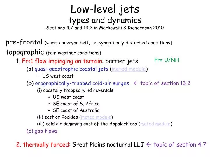
Low-level jets types and dynamics Sections 4.7 and 13.2 in Markowski & Richardson 2010. pre-frontal (warm conveyor belt, i.e. synoptically disturbed conditions) topographic (fair-weather conditions) 1. Fr<1 flow impinging on terrain : barrier jets

E N D
Low-level jets types and dynamicsSections 4.7 and 13.2 in Markowski & Richardson 2010 pre-frontal (warm conveyor belt, i.e. synoptically disturbed conditions) topographic (fair-weather conditions) 1. Fr<1 flow impinging on terrain: barrier jets (a) quasi-geostrophic coastal jets (meted module) • US west coast (b) orographically-trapped cold-air surges topic of section 13.2 (i) coastally trapped wind reversals • US west coast • SE coast of S. Africa • SE coast of Australia (ii) east of Rockies (meted module) (iii) cold air damming east of the Appalachians (meted module) (c) gap flows 2. thermally forced: Great Plains nocturnal LLJ topic of section 4.7 Fr= U/NH
1. Barrier jets (Fr<1): early studies • Schwerdtfeger (1975, 1979) describes a barrier jet along the Antarctic Peninsula. He correctly interprets the dynamics, and estimates the BJ to be ~100 km wide. • Parish (1982) documents and models the BJ in the CA Central Valley. He explains it as an ageostrophic response to the damming of stably-stratified flow by the Sierra Nevada. Evaporation and melting of precip may have enhanced the stratification. T deep cold pool shallow cold pool Vt PGF dv/dt=PGF+CF H CF (Schwerdtfeger 1975) (Parish 1982)
1.a: quasi-geostrophic coastal jets Flight track northerly wind (-v) VT : calculated geostrophic wind profile obtained by adding thermal wind components to lowest-level geostrophic wind Vg warm cold MBL inversion top MBL inversion base west east Parish (2000)
1.a: force balance in west coast jet Vt inversion x T warm cold hot 1 km H CF PGF L W E 200 km z Vt v Ekman?
1.a: coastal jet: summary of dynamics Fr= U/NH • Fr <1 • close to geostrophic balance • the PGF points onshore, to the mountain barrier • on the mesoscale, this PGF is enhanced due to the sharp baroclinicity across the coast (trapped thermally-direct circulation) • this explains the slope of the MBL inversion (lower near the coast) • this slope implies wind shear in opposite direction of the LLJ, i.e. the wind above the LLJ is also ~geostrophic • coastal jets flow to the right of the adjacent barrier in the NH • to the left in the SH, eg in Chile and Namibia • most common in the warm season • large land-sea temperature contrast and thus large onshore PGF • often persistent
1.b: orographically-trapped cold-air surges • (i) coastally-trapped wind reversals Fig. 13.3 (Mass and Albright 1987)
coastally-trapped wind reversals Mass and Bond (1996) Ralph et al (1998)
Normal conditions (coastal jet) preclude southerly winds along the west coast. • Synoptically, a CTWR is preceeded by warm advection and/or subsidence warming (lee troughing) offshore, to the north. This thins the MBL and causes low SLP. • A CTWR is triggered and maintained by an anomalous along-shore pressure gradient. The wind reversal itself can be explained by ageostrophic down-gradient flow, i.e. the disturbance is driven by MBL depth differences. • Full-physics models simulate CTWR rather well (e.g. Rahn and Parish 2007)
1.b(i) CTWR in SE Australia: the Southerly “burster” axis of subtropical high southerly changes most common in late spring
Sydney1 Dec ‘82 southeasterly: onshore Colquhoun et al 1985
Sydney x Melbourne x 1500 m Colquhoun et al 1985
model observations +24 case 1 case 2 McInnes and McBride 1994
potential temperature Uacross x McInnes and McBride 1994
Using a model to explain the ducting of the cold air along the SE coast McInnes and McBride 1994
1.b(ii) orographically-trapped cold-air surges east of the Rockies terrain COMET meted module 19 March 2003 CSU Chill radial velocity location of cross section (next slide)
orographically-trapped cold-air surges east of the Rockies:18 March 2003 case study
1.b: orographically-trapped cold-air surges: dynamics H L H cold-airmass boundary L deflection along-barrier jet retardation Figs. 13.7 and 13.8
synoptic-scale perspective: barrier jet east of the Rocky Mtns, and cold surge into Mexico (b) 3/13 00Z (a) 3/12 12Z (c) 3/13 12Z Schultz et al 1997
N Schultz et al 1997 S
1.b(iii) orographically-trapped cold-air surgescold-air damming east of the Appalachians surface temperatures (F) Figs. 13.6
1.b(iii) orographically-trapped cold-air surgescold-air damming east of the Appalachians Figs. 13.4, 5, 9
1.b: orographically-trapped cold-air surges summary of dynamics • similarities with coastal jet: • Fr <1: terrain blockage • differences with coastal jet: • geostrophic wind towards the mountain, rather than PGF • flow is highly ageostrophic • upslope or onshore flow slows down • PGF exceeds CF, thus flow becomes down-gradient • there is a high close to the mountain ridge, due to • deepening of shallow cold pool (sloping isentropes) • plus possibly CAA associated with poleward anticyclone • plus possibly diabaticcooling (melting/evaporation) • rule of thumb: these barrier jets flow to the left of the terrain that the geostrophic wind impinges upon in the NH. • southbound on east side, northbound on westside of N-S oriented mtn ranges • reverse in the SH • most common in the season of strongest baroclinicity • along coast (CTWR): summer • inland: winter • usually transient
1.c gap winds 20 m/s Marwitz and Dawson 1984
2. thermally-forced LLJs:the fair-weather Great Plains nocturnal LLJ .Vici nocturnal LLJ frequency in 4 summers (Bonner 1968) Fig. 4.32 Fig. 4.31
example wind profiles: 24 hour cycle Fig. 4.35 Rawinsonde wind profiles at Oklahoma ARM CART site on 31 July 1994 (Whiteman et al 1997)
Great Plains southerly vs northerly LLJ climatology for 702 cases of southerly LLJ and 658 cases of northerly LLJ over the ARM-CART site (Whiteman et al 1997) In winter, both N-LLJ and S-LLJ occur under strong synoptic forcing, any time of the day or night. In summer, S-LLJ are far more common, under weak synoptic forcing, strongly diurnally modulated. We are interested in the S-LLJ only
2. thermally-forced LLJs:the fair-weather Great Plains nocturnal LLJ • characteristics: • nighttime only • peaks in strength between midnight and sunrise • wind maximum at 0.5-1.0 km AGL • just above the top of NBL • flow decoupled from surface friction layer • speed: 0-30% stronger than geostrophic wind, peak winds 15-30 m/s • present up to 50% of time in spring/early summer • strongest/most common in central OK/KS • LLJ’s significance for nocturnal elevated convection: • moisture/thermal advection (affects CAPE) • enhanced shear (affects storm organization) • storm severity controlled by both CAPE and shear
thermally-forced LLJ dynamics (a) inertial oscillation period: 2p/f =12 hrs/sinf start near sunset when wind is sub-geostrophic (friction F in the CBL)
Central Great Plains southerly low-level jet: dynamics • first, the persistent southerly geostrophic wind should be noted (Colorado low) • inertial oscillation driven by CBL • winds in convective BL (CBL) subgeostrophic: • assume friction now disappears (nighttime decoupling from NBL) • result is inertial oscillation: • inertial period is 2p/f (f=30°: P=24 hrs; f=45°: P=17 hrs) • wind becomes super-geostrophic, more so if daytime retardation is larger • thermal wind:
Central Great Plains southerly low-level jet: dynamics FA z INV • The zonal temperature gradient and thus the PGF across the sloping Plains varies diurnally • This forces a diurnally-varying acceleration (across-contours) • And this creates a along-contour thermal wind • results in a southerly LLJ at night • this geostrophic adjustment is delayed by a quarter inertial period (4-6 hrs) west CBL east q FA: free atmosphere RCBL: residual CBL NBL: nocturnal BL INV: inversion FA z RCBL east west NBL NBL q
jet east of central Andes is equivalent to southerly Great Plains LLJ SALLJEX 2003 (Vera et al, 2006Great Plains , BAMS 87, 63) Santa Cruz Bolivia Mean 12 Z (dawn) wind profile over Santa Cruz in January (summer) J NW wind
2: Great Plains southerly LLJ summary of dynamics • warm-season, nocturnal, peaks just above NBL • two types of thermal forcing: • daytime heating over elevated terrain produces persistent deep low up there • nighttime cooling over elevated terrain results in geostrophic LLJ • surface heating: CBL retards southerly geostrophic flow during the day • decoupling from the NBL at night results in super-geostrophic flow • turning of wind is an inertial oscillation • rule of thumb: LLJ blows cyclonically around elevated terrain • Altiplano LLJ is a northerly wind (mtns = South American Andes) • I-95 corridor LLJ is a southwesterly wind (mtns = Appalachian) • Coastal NSW LLJ is a N-NE wind (mtns = Dividing Range in Australia) • Lowveld LLJ is a NE wind (mtns = Drakensberg Range in South Africa)
references • Great Plains: • Walters CK, Winkler JA, 2001: Airflow configurations of warm season southerly low-level wind maxima in the Great Plains. Part I: spatial and temporal characteristics and relationship to convection. WEATHER FORECAST 16 (5): 513-530. • Whiteman CD, Bian XD, Zhong SY, 1997: Low-level jet climatology from enhanced rawinsonde observations at a site in the southern Great Plains. J APPL METEOROL 36 (10): 1363-1376. • Helfand HM, Schubert SD, 1995: Climatology of the simulated great-plains low-level jet and its contribution to the continental moisture budget of the United States. J CLIMATE 8 (4): 784-806. • Mark J, Arritt RW, Labas K, 1995: A climatology of the warm-season great-plains low-level jet using wind profiler observations. WEATHER FORECAST 10 (3): 576-591. • Lanicci JM, Warner TT, 1991: A synoptic climatology of the elevated mixed-layer inversion over the southern Great Plains in spring. 3. relationship to severe-storms climatology. WEATHER FORECAST 6 (2): 214-226. • West coast: • Parish TR, 2000: Forcing of the summertime low-leveljet along the California coast. J APPL METEOROL 39 (12): 2421-2433. • Douglas MW, Valdez-Manzanilla A, Cueto RG, 1998: Diurnal variation and horizontal extent of the low-leveljet over the northern Gulf of California. MON WEATHER REV 126 (7): 2017-2025. • Appalachians: • Sjostedt DW, Sigmon JT, Colucci SJ, 1990: The Carolina nocturnal low-leveljet - synoptic climatology and a case-study. WEATHER FORECAST 5 (3): 404-410. • South America, China, South Africa: • Seluchi ME, Marengo JA, 2000: Tropical-midlatitude exchange of air masses during summer and winter in South America: Climatic aspects and examples of intense events. INT J CLIMATOL 20 (10): 1167-1190. • Ding YH, 1992: Summer monsoon rainfalls in China. J METEOROL SOC JPN 70 (1B): 373-396. • Ross KE, Piketh SJ, Swap RJ, et al., 2001: Controls governing airflow over the South African lowveld. S AFR J SCI 97 (1-2): 29-40.