Download
1 / 19
200 likes | 403 Views
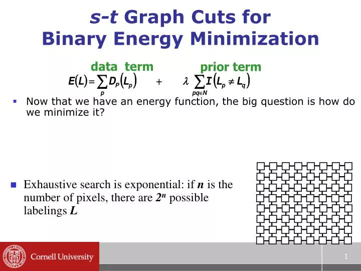
s-t Graph Cuts for Binary Energy Minimization. Now that we have an energy function, the big question is how do we minimize it? . data term. prior term. Exhaustive search is exponential: if n is the number of pixels, there are 2 n possible labelings L. Max flow problem:

E N D
s-t Graph Cuts forBinary Energy Minimization • Now that we have an energy function, the big question is how do we minimize it? data term prior term • Exhaustive search is exponential: if n is the number of pixels, there are 2n possible labelings L
Max flow problem: Each edge is a “pipe” Find the largest flow F of “water” that can be sent from the “source” to the “sink” along the pipes Source output = sink input = flow value Edge weights give the pipe’s capacity a flow F “source” “sink” T S A graph with two terminals Maximum flow problem
Min cut problem: Find the cheapest way to cut the edges so that the “source” is separated from the “sink” Cut edges going from source side to sink side Edge weights now represent cutting “costs” a cut C “source” “sink” T S A graph with two terminals Minimum cut problem
Max Flow = Min Cut: Proof sketch: value of a flow is value over any cut Maximum flow saturates the edges along the minimum cut Ford and Fulkerson, 1962 Problem reduction! Ford and Fulkerson gave first polynomial time algorithm for globally optimal solution “source” “sink” T S A graph with two terminals Max flow/Min cut theorem
Fast algorithms for min cut • Max flow problem can be solved fast • Many algorithms, we’ll sketch one • This is not at all obvious • Variants of min cut are NP-hard • Multiway cut problem • More than 2 terminals • Find lowest cost edges separating them all
“source” “sink” T S A graph with two terminals “Augmenting Path” algorithms • Find a path from S to T along non-saturated edges • Increase flow along this path until some edge saturates
“source” “sink” T S A graph with two terminals “Augmenting Path” algorithms • Find a path from S to T along non-saturated edges • Increase flow along this path until some edge saturates • Find next path… • Increase flow…
“source” “sink” T S A graph with two terminals “Augmenting Path” algorithms • Find a path from S to T along non-saturated edges • Increase flow along this path until some edge saturates Iterate until … all paths from S to T have at least one saturated edge
Implementation notes • There are many fast flow algorithms • Augmenting paths depends on ordering • Breadth first = Edmonds-Karp • Vision problems have many short paths • Subtleties needed due to directed edges • [BK ’04] gives an algorithm especially for vision problems • Software is freely available
a cut Dp(0) t s Dp(1) Basic construction • One non-terminal vertex per pixel • Each pixel connects directly to s,t • Severing these edges corresponds to giving labels 0,1 to the pixel • Cost of cut is the cost of the entire labeling
p p r q s s q • The cut in red corresponds to labeling black r 0 • The cut in green corresponds to labeling 1 white Example • For clarity, let’s look at 1 dimensional example but everything works in 2 or higher dimensions. Suppose our image has 4 pixels: • We build a graph:
Beyond binary faxes • All we really need is a cost function • Suppose that label 1 means “foreground” and label 0 means “background” • How do we figure out if a pixel prefers to be in the foreground or background? • Predefined intensities: for instance, the foreground object tends to have intensities in the range 50-75 • So if we observed an intensity in this range at p, Dp(1) is small • This is not image thresholding!
Better intensity models • We can compute the range of intensities dynamically rather than statically • Both for foreground and for background • User marks some pixels as being foreground, and some as background • Compute a Dpbased on this • For instance, Dp(1) is small if p looks like pixels marked as being foreground • Based on the resulting segmentation, mark additional pixels
A serious implementation • This basic segmentation algorithm is now in a Microsoft product • SIGGRAPH paper on “GrabCut” • Same basic idea, but simpler UI • Assume the background is outside and the foreground is inside a user-supplied box • Dp(1) is small if p looks like the pixels inside the box, large if like the pixels outside • Create a new segmentation and use it to re-estimate foreground and background
GrabCut – Interactive Foreground Extraction Iterated Graph Cuts Guaranteed toconverge 1 3 4 2 Result See: http://www.youtube.com/watch?v=9jNB6fza0nA&feature=related
GrabCut – Interactive Foreground Extraction Moderately straightforward examples … GrabCut completes automatically
Important properties • Very efficient in practice • Lots of short paths, so roughly linear • Construction is symmetric (0 vs 1) • Specific to 2 labels • Min cut with >2 labels is NP-hard
Can this be generalized? • NP-hard for Potts model [K/BVZ 01] • Two main approaches 1. Exact solution [Ishikawa 03] • Large graph, convex V (arbitrary D) • Not the considered the right prior for vision 2. Approximate solutions [BVZ 01] • Solve a binary labeling problem, repeatedly • Expansion move algorithm