Download
1 / 42
430 likes | 771 Views
What Energy Functions Can be Minimized Using Graph Cuts?. Shai Bagon Advanced Topics in Computer Vision June 2010. What is an Energy Function?. Image Segmentation:. For a given problem:. Useful Energy function: Good solution Low energy Tractable Can be minimized .

E N D
What Energy Functions Can be Minimized UsingGraph Cuts? Shai Bagon Advanced Topics in Computer Vision June 2010
What is an Energy Function? Image Segmentation: For a given problem: • Useful Energy function: • Good solution Low energy • Tractable Can be minimized suggested solution E a number -20 237
Families of Functions orOutline • F2 submodular • Non submodular • F3 • Beyond F3
Foreground Selection yi xi xm xn Let yi – color of ith pixel xiϵ {0,1}BG/FG labels (variables) Given BG/FG scribbles: Pr(xi|yi)=How likely each pixel to be FG/BG Pr(xm|xn)=Adjacent pixels should have same label F2 energy: E(x)=∑iEi(xi)+∑ijEij(xi,xj)
Submodular Known concept from set-functions: E(x) = ∑i Ei(xi) + ∑ij Eij (xi, xj), xiϵ {0,1} What does it mean? 0 1 xj xi 0 A B Eij(xi,xj): B+C-A-D ≥ 0 1 C D
F2 submodular How toMinimize? E(x) = ∑i Ei(xi) + ∑ij Eij (xi, xj), xiϵ {0,1} Local “beliefs”: Data term Prior knowledge:Smoothness term
Graph Partitioning Ì Ì Î Î S V , T V , s S , t T Ç = f È = S T , S T V å = Cut ( S , T ) wij Î Î i S , j T V A weighted graph G=( V E w ) Special Nodes:st s-t cut: Cost of a cut: Nice property: 1:1 mapping s-t cut↔ {0,1}|V|-2 E w s wij t
Graph Partitioning Graph Partitioning - Energy Eij(xi,xj) xj xi 0 1 0 A B 0 0 0 D-C 0 B+C-A-D = A + + + 1 C D C-A C-A 0 D-C 0 0 D-C C-A E(x) = ∑i Ei(xi) + ∑ij Eij (xi, xj) s Ej(1) B+C-A-D j i Ei(0) t
Graph Partitioning Graph Partitioning - Energy D-C C-A E(x) = ∑i Ei(xi) + ∑ij Eij (xi, xj) s Ej(1) st cut binary assignment cut cost energy of assignment min cut Energy min. B+C-A-D j i Ei(0) t B=Eij(0,1)
Recap F2 submodular: E(x) = ∑i Ei(xi) + ∑ij Eij (xi, xj) Eij(1,0)+Eij(0,1)≥Eij(0,0)+Eij(1,1) Mapping from energy to graph partition Min Energy = computing min-cut Global optimum in poly timefor submodular functions!
Next… Multi-label F2 E(x)=∑i Ei(xi) + ∑ij Eij(xi,xj) s.t. xi ϵ{1,…,L} • Fusion moves: solving binary sub-problems • Applications to stereo, stitching, segmentation… Solve Binary problem: xi=0 xi=1 ● = Fusion Current labeling suggested labeling “Alpha expansion”
Stereo matching see http://vision.middlebury.edu/stereo/ Input: Pairwise MRF [Boykov et al. ‘01] Ground truth slide by Carsten Rother, ICCV’09
Panoramic stitching slide by Carsten Rother, ICCV’09
Panoramic stitching slide by Pushmeet Kohli, ICCV’09
AutoCollage [Rother et. al. Siggraph ‘05 ] http://research.microsoft.com/en-us/um/cambridge/projects/autocollage/
Next… Multi-label F2 E(x)=∑i Ei(xi) + ∑ij Eij(xi,xj) s.t. xi ϵ{1,…,L} • Fusion moves: solving binary sub-problems • Applications to stereo, stitching, segmentation… Non-submodular Beyond pair-wise interactions: F3
Merging Regions regions (Ncuts) input image “edge” prob. j i pi “weak” edge pi – prob. of boundary being edge GOAL: Find labeling xiϵ{0,1} that max: min: “strong” edge Taking -log
Merging Regions Adding and subtracting the same number
Merging Regions x1 x2 x3 EJ 0 0 0 0 1 1 1 0 0 1 1 0 0 0 1 λ Solving for edges: Consistency constraints:No “dangling” edge J xi wi No longer pair-wise: F3
Minimization trick Freedman D., Turek MW, Graph cuts with many pixel interactions: theory and applications to shape modeling. Image Vision Computing 2010
Merging Regions The resulting energy: + Pair-wise - Non submodular!
Quadratic Pseudo-Boolean Optimization j t i s j i Kolmogorov V., Carsten R., Minimizing non-submodular functions with graph cuts – a review. PAMI’07
Quadratic Pseudo-Boolean Optimization j i + All edges with positive capacities - No constraint Labeling rule: partial labeling s j i t
Quadratic Pseudo-Boolean Optimization j i Properties of partial labeling y: 1. Let z=FUSE(y,x)E(z)≤E(x) 2. y is subset of optimal y* y is complete: 1. E submodular 2. Exists flipping (inference in trees) s j i t
QBPO - Probing QPBO: p p p q q q r r r s s s t t t 0 1 Probe Node p: • What can we say about variables? • r -> is always 0 • s -> is always equal to q • t -> is 0 when q = 1 slide by Pushmeet Kohli, ICCV’09
QBPO - Probing • Probe nodes in an order until energy unchanged • Simplified energy preserves global optimality and (sometimes) gives the global minimum slide by Pushmeet Kohli, ICCV’09
Merging Regions Result using QPBO-P: input image regions (Ncuts) Result
Recap • F3 and more • Minimization trick • Non submodular • QPBO approx. – partial labeling
Beyond F3… [Kohli et. al. CVPR ‘07, ‘08, PAMI ’08, IJCV ‘09]
Image Segmentation n = number of pixels E: {0,1}n→R 0 →fg, 1→bg E(X) = ∑ ci xi + ∑dij |xi-xj| i i,j Image Segmentation Unary Cost [Boykov and Jolly ‘ 01] [Blake et al. ‘04] [Rother et al.`04]
Pn Potts Potentials Patch Dictionary (Tree) { 0 if xi = 0, i ϵ p Cmax otherwise h(Xp) = Cmax 0 p • [slide credits: Kohli]
Pn Potts Potentials n = number of pixels E: {0,1}n→R 0 →fg, 1→bg E(X) = ∑ ci xi+ ∑dij |xi-xj| +∑ hp (Xp) i i,j p { 0 if xi = 0, i ϵ p Cmax otherwise h(Xp) = p • [slide credits: Kohli]
Image Segmentation n = number of pixels E: {0,1}n→R 0 →fg, 1→bg E(X) = ∑ ci xi+ ∑dij |xi-xj| +∑ hp (Xp) i i,j p Image Pairwise Segmentation Final Segmentation • [slide credits: Kohli]
Application: Recognition and Segmentation One super-pixelization Image another super-pixelization Pairwise CRF only[Shotton et al. ‘06] Pn Potts Unaries onlyTextonBoost[Shotton et al. ‘06] • from [Kohli et al. ‘08]
Robust(soft) Pn Potts model p Pn Potts Robust Pn Potts { 0 if xi = 0, i ϵ p f(∑xp) otherwise h(xp) = p • from [Kohli et al. ‘08]
Application: Recognition and Segmentation another super-pixelization Image One super-pixelization robust Pn Potts (different f) robust Pn Potts Pairwise CRF only[Shotton et al. ‘06] Pn Potts Unaries onlyTextonBoost[Shotton et al. ‘06] • From [Kohli et al. ‘08]
Same idea for surface-based stereo[Bleyer ‘10] Stereo with robust Pn Potts One input image Ground truth depth Stereo with hard-segmentation This approach gets best result on Middlebury Teddy image-pair:
How is it done… Most general binary function: H (X) = F ( ∑ xi) concave H (X) 0 ∑ xi The transformation is to a submodular pair-wise MRF, hence optimization globally optimal • [slide credits: Kohli]
Higher order to Quadratic { 0 if all xi = 0 C1 otherwise x ϵ {0,1}n f(x) = minC1a + C1 (1-a)∑xi = minf(x) x x,a ϵ{0,1} Higher Order Function Quadratic Submodular Function ∑xi = 0 a=0 f(x) = 0 ∑xi > 0 f(x) = C1 a=1 Start with Pn Potts model: • [slide credits: Kohli]
Higher order to Quadratic minC1a + C1 (1-a) ∑xi = minf(x) x x,a ϵ{0,1} Higher Order Function Quadratic Submodular Function C1∑xi C1 1 2 3 ∑xi • [slide credits: Kohli]
Higher order to Quadratic minC1a + C1 (1-a) ∑xi = minf(x) x x,a ϵ{0,1} Higher Order Submodular Function Quadratic Submodular Function C1∑xi a=1 a=0 Lower envelope of concave functions is concave C1 1 2 3 ∑xi • [slide credits: Kohli]
Summary s j i j f2(x) i a=1 a=0 f1(x) t ∑xi • Submodular F2 • F3 and beyond: minimization trick • Non submodular • QPBO(P) • Beyond F3 – Robust HOP Thank You!