Mean Motion Resonances

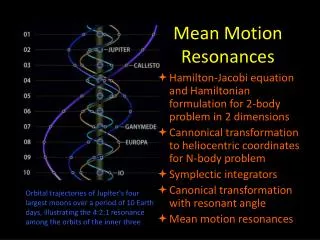
1. Mean Motion Resonances Hamilton-Jacobi equation and Hamiltonian formulation for 2-body problem in 2 dimensions Cannonical transformation to heliocentric coordinates for N-body problem Symplectic integrators Canonical transformation with resonant angle Mean motion resonances Orbital trajectories of Jupiter's four largest moons over a period of 10 Earth days, illustrating the 4:2:1 resonance among the orbits of the inner three

2. Integrable motion • Integrable: n degree of freedom Hamiltonian has n conserved quantities • Examples: • Hamiltonian is a function of coordinates only • Hamiltonian is a function of momenta only – in this case we can call the momenta action variables and we can say we have transformed to action angle variables • Hamiltonian has 1 degree of freedom and is time independent. H(x,v) gives level contours and motion is along level contours. • Arnold-Louiville theorem - integrable implies that the Hamiltonian can be transformed to depend only on actions

3. Hamilton Jacobi equation • If the coordinate q does not appear in the Hamiltonian then the corresponding momentum p is constant • Try to find a Hamiltonian that vanishes altogether, then everything is conserved • Generating function S2(q1,q2,…;P1, P2, …,t) function of old coordinates and new momenta which we would like conserved • New Hamiltonian

4. Finding conserved momenta 2-body problem • Our new momenta are conserved, constants of integration, Pi • 2 body in 2 dimensions • Hamilton Jacobi equation old coordinates new momenta

5. Assume separable • Substitute momenta in to Hamilton Jacobi equation • Since separable • Hamilton Jacobi equation gives Because we choose S separable these derivatives must be constant, as they are constant we also make them be our new momenta

6. S depends on new monenta so α1α2 are new momenta using expression for L is energy New coordinates

7. Sub in for constants and use Q1 is time of perihelion

8. (Hamilton Jacobi equation and 2 body problem continued) • With a similar integral we can show that Q2 is angle of perihelion • 3D problem done similarly • These coordinates not necessarily ideal. Add and subtract them to find the Delaunay, modified Delauney and Poincaré coordinates

9. Cannonical transformations Different approaches • Choose desirable generating functions • Solve integrals resulting from Hamilton-Jacobi equation • Choose new coordinates and momenta and show they satisfy Poisson brackets • Use expansions (e.g., Birkhoff normal form) (can lead to problems with small divisors)

10. Example(continuing two body problem) Desirable to have a third angle as a coordinate The mean anomaly M = n(t-τ) as expected

11. Harmonic oscillator • Use Poisson bracket to check that these variables are cannonical you don’t get 1 here unless there is the factor of 2 in the variable

12. Harmonic oscillator Using a generating function

13. Heliocentric coordinates N-bodies in inertial frame generating function new Hamiltonian

14. Democratic heliocentric coordinate system • If P0=0 Hamiltonian becomes barycenter so can be set to zero This is equivalent to using momenta that are in center of mass coordinate system Keplerian term Interaction term Drift term

15. Democratic heliocentric coordinates • Hamiltonian is nicely separable in • heliocentric coordinates and • barycentric momenta

16. Jacobi Coordinates To add a body: work with respect to center of mass of all previous bodies. Coordinate system requires a tree to define.

17. Symplectic Integrators • Wisdom and Holman used a Hamiltonian in Jacobi coordinates for the N-body system that also separated into Keplerian and Interaction terms. • Hamiltonian approximated by • Integrated all bodies with f,g functions for dt = 1/Ω (that’s Hkep) • Velocities given a kick caused by Interactions • Integrate bodies again with f,g functions dt = 1/Ω • Integrator is symplectic but integrates a Hamiltonian that approximates the real one. • The integrator has bounded energy error and allows very large step sizes

18. Second order Symplectic integrator Poisson bracket with H gives evolution Find coefficients so this is true to whatever order you desire (see Yoshida review)

19. Second order Symplectic integrator Expand to second order ~ =

20. Second order for N-body • Evolve Kepsteps via f,g functions • Drift step lets positions change as the Hamiltonian term only depends on momenta • Interaction steps only vary velocities as they only depend on coordinates • Reverse order. • Central step chosen to be most computationally intensive • This is known as the democratic heliocentric second order integrator (Duncan, Levison & Lee 1998)

21. Symplectic integrators- Harmonic oscillator • The exact solution is • To first order in τ • However and energy increases with time • A symplectic scheme can be constructed with

22. More on symplectic integrators • This is symplectic because the det is 1 and so volume is conserved • There is a conserved quantity but it’s not the original Hamiltonian • You can show this by computing this quantity for p’,q’ • The difference between new and old Hamiltonian depends on timestep! • Integrator is no longer symplectic if timestep varied.

23. Approximating interactions with Periodic delta functions • Interaction terms are used to perturb the system every time step • Class of integrators where fast moving terms are replaced with periodic delta function terms. • Note interaction term only depends on coordinates. • Here is an example: • We add extra terms to interaction term periodic function

24. Integrating the approximate Hamiltonian • For t≠2πn • For t=0,2π,4π… • Integrate over the delta function • Procedure: integrate unperturbed Hamiltonian between delta function spikes. At each t=0,2π,4π… update momenta. These are the velocity kicks.

25. Justifications • Often the Hamiltonian has many cosine terms. As long as frequencies are not commensurate, a perturbative transformation can remove non-resonant terms. Dynamics is only weakly sinusoidally varied by these terms. Cosine terms that are not commensurate are ignored. • We can add in cosine terms without significantly changing the dynamics. • The approximate Hamiltonian is conserved exactly. • Sizes of errors can be quantified. Errors are bounded as there is a conserved quantity. • You can’t change the step size as this would change the approximate Hamiltonian integrated. If you change the step size, the bounded property of errors is lost. • Wisdom, Holman, and collaborators

26. Similarity to Standard map • I, θ mod 2π • If constant K is small there is no chaos. • Width of chaotic zone depends on K • Above a certain value of K -> global chaos

27. Regularization Given • Hamiltonian H(p,q) • Initial conditions H(p0,q0,t=0)=H0 Let We have a new Hamiltonian system but time can be re-scaled Symplectic integrators that require equal timesteps can be constructed with the new time variable `Extended phase space’ using time to deal with initial conditions issue

28. General view of resonance vector of integers k such that Contrast with Periodic orbits a period T such that for every frequency ωi is close to an integer Zi T is a multiple of the period of oscillation for every angle

29. Small divisor problem frequencies expand perturbation in Fourier series We would like to find new variables similar to the old variables try this and try to find nice values for ck Canonical transformation Insert this back into Hamiltonian Choose These can be small!

30. Small divisor problem continued first order perturbations removed Nearing a resonance, the momentum goes to infinity We will see that the infinity is not real, but a result of our assumption that new and old variables are similar If there are no small divisors when removing first order perturbations, there may be small divisors when attempting to remove higher order perturbations from Hamiltonian via canonical transformation

31. Using the resonant angle generating function resonant angle is a new coordinate n-1 conserved quantitiesJibecause Hamiltonian lacks associated angles Can expand H0 in orders of J0

32. Resonant angle Simple 2D Hamiltonian. There is no infinity in the problem. Dynamics is similar to that of the pendulum. We did not assume that all new angles were similar to old angles in the transformation. The infinite response previously seen near resonance was caused by the choice of coordinate system Above we considered only a single cosine term When there is more than one cosine term, then dynamics can be more complicated Adopt a condition that the system is always sufficiently far from resonance, allowing perturbation theory to be done at all orders (Kolmogorov approach) Consider proximity of resonances (Chirikov approach)

33. Expanding about a mean motion resonance (Celestial mechanics) • j:j-k resonance exterior to a planet • generating function • new momenta unperturbed Hamiltonian units μ=1 mean longitude of planet ψ is resonant angle

34. Expand around resonance with coefficients

35. Adding in resonant terms from the disturbing function secular term have opposite signs

36. First order resonances sets distance to resonance corotation term proportional to planet eccentricity usually dropped but can be a source of resonance overlap + chaos (Holman, Murray papers in 96)

37. One last C-transformation and going down a dimension New Hamiltonian has no second angle so J2is conserved We can ignore it in dynamics It may be useful to remember J2 later to relate changes in eccentricity to changes in semi-major axis in the resonance

38. Distance to Resonance, Pendulum Hamiltonian transformed to a pendulum Hamiltonian but with momentum shifted fixed point is shifted

39. Dimensional analysis • Units of H cm2/s2 Units of Γ cm2/s • Units of a cm-2 Units of δ cm s-3/2 • δ2 × a units s-3 • Unit of time a-1/3 δ-2/3 sets typical libration period • δ2/3 units cm2/3 s-1 • Unit of momentum δ2/3a-2/3 sets resonant widths • δ is proportional to Planet mass • Resonant widths depend on planet mass to the 2/3 power. • Migration is a variation in mean motion so has units s-2 • Relevant to figure out adiabatic limit

40. As distance to resonance varied coordinate system • Only one side has a separatrix • On one side it looks like a harmonic oscillator • 3 fixed points but only 2 stable • Without circulating about origin means in resonance • Can think of drifting problems as having time dependent b

41. Drifting systems • Migrating planets • Dust under radiation forces (though dissipative dynamics is NOT Hamiltonian) • Satellite systems with tidal dissipation

42. Drifting systems Particle must jump to other side, no capture possible Particle can be pumped to high eccentricity and remain in librating island, resonance capture possible

43. Production of Star Grazing and Star-Impacting Planetesimals via Planetary Orbital MigrationQuillen & Holman 2000, but also see Quillen 2002 on the Hyades metallicity scatter Numerical integration of a planet migrating inwards Eject Impact FEB

44. Integration with toy model Escape resonant angle fixed -- Capture

45. Failure to capture • Volume in resonance shrinking rather than growing (particle separating from planet) • Non-adiabatic limit. Rapid drifting • Initial particle eccentricity is high. • Prevented by strong subresonances

46. Adiabatic Capture Theoryfor Integrable Drifting Resonances Theory introduced by Yoder and Henrard, applied toward mean motion resonances by Borderies and Goldreich

47. Critical eccentricity • Below a critical eccentricity probability of capture is 100% • This eccentricity can be estimated via dimensional analysis from the typical momentum size scale in the resonance • It depends on order of resonance and a power of planet mass. Hence weak resonances require extremely low eccentricity for capture. • Exact probability above ecrit in adiabatic limit can be computed via area integrals

48. Limitations of Adiabatic theory • At fast drift rates resonances can fail to capture -- the non-adiabatic regime. • Subterms in resonances can cause chaotic motion. temporary capture in a chaotic system

49. Coupled pendulum • plot points every t=1/ν to make a surface of section • 2D system (4D phase space) can be plotted in 2D with area preserving map • Nice work relating timescales for evolution to overlap parameter by Holman and Murray forced pendulum analogous first order resonance system

50. Chaos first develops near separatrix chaotic orbits more likely on this side