Download
1 / 56
570 likes | 575 Views
ITEP Winter School, 13-20 Feb 2010. New charmonium resonances. Roman Mizuk, ITEP. Outline. Potential Models. Traditional charmonium states. New charmonium resonances. X(3872) 1 - - states from ISR 3940 family Z ±. Bottomonium. meson containing cc quarks. Charmonium –.

E N D
ITEP Winter School, 13-20 Feb 2010 New charmonium resonances Roman Mizuk, ITEP
Outline Potential Models Traditional charmonium states New charmonium resonances X(3872) 1- - states from ISR 3940 family Z± Bottomonium
meson containing cc quarks Charmonium – Family of excited states: c , J/ , cJ , hc , (2S) , … “Hydrogen atom” of QCD Basic properties of most states simple picture of non-relativistic cc pair.
non-relativistic relativistic Quantum Mechanics Quantum Field Theory Number of particles is not conserved multi-body problem two-body problem
Hydrogen atom non-relativistic Srödinger equation relativistic bispinor Dirac equation Precise description of hydrogen atom. EXCEPT FOR LAMB SHIFT.
Field Theoretical description of bound state e- + + + … Amplitude: p Analytic continuation into complex energy plane. Im E Re E mp+me poles bound states
Hydrogen atom (2) Solutions of Dirac equationcorrespond to sum + + + … + … = running charge, distorts Coulomb potential too small effect to reproduce Lamb shift + … reproduces Lamb shift No way to account for in Dirac equation. not a single particle! Non-potential effects are small if electron is slow in the time scale when additional degrees of freedom are present in the system. ~ = v/c
Potential Model of Charmonium + + … = constituent quark, heavier by 300MeV QCD motivated potential + + … Assume that charm quark is heavy enough to neglect non-potential effects. + … (M(2S) – MJ/ ) / QCD = 590 MeV / 200 MeV Not justified: is not small. Open question: why Potential Models work reasonably well for charmonium?
Charmonium Potentials c J/ c2 (2S) “Cornel model” one-gluon exchange, asymptotic freedom confiningpotential, “chromoelectric tube” There are other parameterizations, respecting or not respectingQCD asymptotics. After parameters of potential are fit to data, the potentials become very similar. 0.1<R<1fm
Charmonium levels without spin 2s 1p 2s 1d 1p Harmonic oscillator Coulomb 1s 1s 2s 1p 1s QCD
Relativistic Corrections fine structure of states spin-singlet triplet splitting not commute with short distance confining Assign Lorentz structure to potentials vector scalar Breit-Fermi expansion to order v2/c2
Charmonium Levels M, GeV building blocks 4.50 P = (–1)L+1 C = (–1)L+S S = s1 + s2 = { 0, 1 } J = S + L n – radial quantum number (4415) 4.25 (4160) spectroscopic notation conserved QN (4040) n(2S+1)LJ JPC c2(2S) 4.00 (3770) c , c(2S) 0– + 1S0 S=0 L=0 3.75 c(2S) (2S) J/ , (2S) , (4040) , (4415) c2 hc 3S1 1– – S=1 L=0 c1 3.50 c0 hc 1P1 1+ – S=0 L=1 3.25 c0 c1 c2 , c2 (2S) 3P1 3P2 3P3 0+ + 1+ + 2+ + J/ S=1 L=1 c 3.00 S=1 L=2 3D1 1– – (3770), (4160) 2.75 (3770) = 13D1 + 0.2 23S1 “S - D mixing” 0– + 1– – 1+ – (0,1,2)+ + JPC
State Experim Predictions of Potential Models
Predictions of Potential Models M, GeV Potential models reproduce also annihilation widths J/y, y(2S)→ℓ+ℓ- hc, ccJ→ ggand radiative transitions btw. charmonia. JPC
Hadronic mass in Lattice QCD from first principles Calculate 2-point Green function G(t,0) = 0O(t)O(0)+0,creating hadron at time 0 and destroying at time t. For this Average over all possible configurations of fields generated on lattice and weighted with exp(iS). → exp(–S) Operator O has required quantum numbers: JPC, flavor contentand is projected on zero momentum. Minkovsky → pseudo-Euclidian space. 2nd radial excitation 1st radial excitation ground state Expect: G(t,0) = A1exp(im1t) + A2exp(im2t) + A3exp(im3t) + ... → A1exp(–m1t) + A2exp(–m2t) + A3exp(–m3t) + ... Multi exponential t-dependence of Green function complicates identification of excited states.
Charmonium in Lattice QCD Potential for static charm quarks. Shape is similar to that of phenomenological models. quenched approximation Predictions for charmonia up to the 1st radial excitation exist.Still a lot of room for improvement.
QCD Sum Rules Green function is calculated analytically. Restricted to small interval of t, contributions from ground and higher states more difficult to resolve. Application restricted to lowest states only.
Summary on Potential Models – Only model relation to underlying fundamental theory of QCD. difficult to assign uncertainties to results + Using 3-4 parameters can describe a lot of data. right choice of variables? good predictive power o In many cases the only available theoretical approach. higher resonances Shape of potential in agreement with Lattice QCD estimations, and with perturbative QCD calculations (at small distances). success of phenomenology Useful framework for refining our understanding of QCDand guidance towards progress in quarkonium physics.
Observation of J/ BNL AGS extracted 28 GeV p-beam SLAC SPEAR e+e- annihilation Mark I first 4 detector Be target Richter et al. , nb , nb p + Be → e+e- + X Ting et al. , nb E c.m.s. Width of t J/ is very narrow, JPC=1– –. M( e+e- )
“Heavy but very narrow !” November 1974 revolution. Every possible explanation was suggested. Observation of charm quark. Quarks generally recognized as fundamental particles. Charm quark was predicted by GIM mechanism to cancel divergence in kaon box diagram.
Observation of (2S) two weeks after observation of J/ SLAC SPEAR Mark I Event Display y(2S) → J/yp+p-J/y→ e+e- (2S) is very narrow, JPC=1– –.
cJ c – DASP, DESY (1976)– Crystall Ball, SLAC (1980) Observation of hc – DASP (1977) hc(2S) – CBall (1980) Crystal Ball: sphere with 900 NaI crystals
First results on R above DD threshold – SPEAR (1975). 4 peaks above 3.7 GeV :
c g g c e,m,q c g e,m,q ¯ ‾ ‾ ‾ c c c Why J/ is so narrow? C-parity 2/3 1/3 DD* D*D* ~as3 DD at threshold For J/ strong decays are suppressed so much that EM decays are competitive.
Charmonium level scheme after 1980 10 states were observed: • 6 ’s directly produced in e+e– annihilation. • 3 P-levels are well seen in (2S) radiative transitions. • The ground state c was observed in radiative decays of J/ and (2S). Charmonium level scheme before 2002
B-factories Instrumented Flux Return (IFR) [Iron interleaved with RPCs]. Superconducting Coil (1.5T) Silicon Vertex Tracker (SVT) e+ (3 GeV) e– (9 GeV) CsI(Tl) Calorimeter (EMC) [6580 crystals]. Cherenkov Detector (DIRC) [144 quartz bars, 11000 PMTs] Aerogel Cherenkov cnt. n=1.015~1.030 Drift Chamber [40 stereo lyrs](DCH) SC solenoid 1.5T 3.5GeV e+ CsI(Tl) 16X0 TOF counter 8GeV e– Tracking + dE/dx small cell + He/C2H5 pp collider CDF D0 E ~ 1.8 TeV ¯ m / KL detection 14/15 lyr. RPC+Fe Si vtx. det. 3 lyr. DSSD e+e–→Y(4S) BaBar Belle E=10.6GeV L~ 2*1034/cm2/s 530 + 1000 fb-1 e+e– → сharmonium CLEO-c BES-II E = 3.0 - 4.8 GeV L ~ 1033/cm2/s
Charmonium production at B factories in B decays γγfusion Any quantum numbers can be produced, to be determined from angular analysis. JPC = 0±+, 2±+ double charmonium production initial state radiation OnlyJPC = 0±+ observed so far. JPC = 1– –
Reconstruction of B decays • In (4S) decays B are produced almost at rest. • ∆E = Ei - ECM/2Signal peaks at 0. • Mbc = { (ECM/2)2 - (Pi)2}1/2Signal peaks at B mass (5.28GeV). B0J/ KS ∆E, GeV Mbc, GeV
Observation of c(2S) B (KSK) K Belle (2002) in B decays and in double charmonium production. Confirmed by BaBar and CLEO-c in two-photon production, and by BaBar in double charmonium production. M = 2654 6 8 MeV/c2 < 55 MeV c(2S) M = 2630 12 MeV/c2 e+e– J/ X Good agreement with potential modelsfor mass, width and 2-photon width. Width: 6±12 (CLEO) and 17± 8 MeV (BaBar) average Γ = (14 ± 7) MeV
Observation of hc y(2S) → p0hc→ p0ghc hc M(hc) = (3524.4 ± 0.6 ± 0.4) MeV < 1 MeV Potential model expectations: M(hc) = centre of gravity of χc states = 1/9 * [(2*2+1) * M(χc2) + (2*1+1) * M(χc1) + (2*0+1) * M(χc0) ] = 3525.3 ± 0.3 MeV
c2(2S) in interactions χс2’ e+ e+ γ D γ D e– e– 395fb-1 5.5 2005, BELLE M=393142MeV/c2 =2083MeV Поляризация consistent with J=2 J=0 disfavored 2/dof=23.4/9 2009, BaBar Width and 2-photon width are in good agreement with models, mass is 50 MeV lower.
Charmonium Levels 2010 DD (2S+1)LJ Y Mass (MeV) y(4415) y(4160) New: y(4040) 3 identified charmonia. c’c2 X Y X y(3770) ~10 states with – mass – decay pattern – quantum numbers that do not fit expectations. h’c y′ cc2 cc1 hc hc cc0 J/y hc (Potential Models) ?? JPC
New charmonium(like) states XYZ resonances states contain cc
– c π c π About 10 charmonium(like) states do not fit expectations. Have Potential Models finally failed? yes, but coupled channel effect was taken into account Exotics? tetraquark molecule two loosely boundD mesons compact diquark-diantiquark state hybrid hadrocharmonium state with excited qluonicdegree of freedom charmonium embeddedinto light hadron
CP X(3872) B→Xsγ 487 Belle citation count 480 336 Phys.Rev.Lett.91262001, (2003) 7th anniversary!
pp collisions PRL91,262001 (2003) X(3872) was observed by Belle in B+ → K+ X(3872) (2S) → J/ψπ+π- X(3872) Confirmed by CDF, D0 and BaBar. Recent signals of X(3872) → J/ψπ+π- direct productiononly 16% from B PRL103,152001(2009) PRL93,162002(2004) arXiv:0809.1224 PRD 77,111101 (2008)
Mass & Width M = 3871.52 0.20 MeV, Γ = 1.3 0.6 MeV Close to D*0D0 threshold: m = –0.42 0.39 MeV [ – 0.92, 0.08 ] MeV at 90% C.L.
Branching Fractions PRL96,052002(2006) (8.10 0.92 0.66) 10-6 (8.4 1.5 0.7) 10-6 Br(B+ X K+) Br(X J/+ -) = Absolute Br? missing mass technique K+ reconstruct only Xcc B+ mX2=(pB+ – pK+)2 (4S) B- (4S) 4-momentumfrom beam energy K+ momentum in B+ c.m.s. Br(B+ X K+) < 3.210–4 at 90%C.L. Br(X J/+ -) > 2.5%
Radiative Decays & J/ hep-ex/0505037 PRL102,132001(2009) J/ J/ (2S) X(3872) → J/+ - 0 subthreshold production of +-0 CX(3872) = +
X(3872) → J/+- Isospin (+-) = 1 L(+-) = 1 CX(3872) = + C+-= – IJPC of 0 (|+1,-1– |-1,+1) ( r ) isospin M (+-) PRL96,102002(2006) hep-ex/0505038 L=0 L=1 M (+-) is well described by 0→+- (CDF: + small interfering →+-). X(3872) → J/ +-X(3872) → J/0
Spin & Parity Br(X → (2S)γ) / Br(X → J/ γ) ~ 3multipole suppression Observation of D*0D0 decaycentrifugal barrier at the threshold PRL98,132002(2007) Angular analyses by Belle and CDF excluded JP = 0++, 0+-, 0-+,1-+ ,1+-, 1--, 2++, 2-- , 2+-, 3--, 3+- 2-+ 1++ 1-- JPC =1++or 2–+ 0++ 2–+is disfavored by JP =1++ are favorite quantum numbers for X(3872). 2–+ not excluded.
X(3872) → D*0D0 PRD77,011102(2008) B+& B0D0D*0K 4.9σ 347fb-1 arXiv:0810.0358 B KD0D*0 D*→Dγ D*→D0π0 605 fb-1 Flatte vs BW similar result: 8.8σ ~2 Shifted X(3872) massin D*D final stateinfluence of nearby D*D threshold.
X(3872) Experimental Summary JPC = 1++(2–+ not excluded) M = 3871.52 0.20 MeV , Γ = 1.3 0.6 MeV Close to D*0D0 threshold: m = – 0.42 0.39 MeV. Br(X(3872) J/0) > 2.5% (90% C.L.)
Br(c1′→J/ )Br(c1′→J/+-) Is there cc assignment for X(3872)? JPC = 1++c1′ ~100 MeV lighter than expected 1++ 2-+ expect 30 measure 0.170.05 3872 JPC = 2–+ηc2 Expected to decay into light hadronsrather than into isospin violating mode. X(3872) is not conventional charmonium.
PRD71,031501,2005 B0 B- X(3872)– X(3872)– M(J/π–π0) M(J/π–π0) Tetraquark? PRD71,014028(2005) [cu][cu] Maiani, Polosa, Riquer, Piccini; Ebert, Faustov, Galkin; … [cq][cq] [cd][cd] [cu][cd] Predictions: Charged partners of X(3872). Two neutral states ∆M = 8 3 MeV,one populate B+ decay, the other B0. Charged partner of X(3872)? No evidence for X–(3872) J/–0 excludes isovector hypothesis
X(3872) Production in B0 vs. B+ B0→XK0s arXiv:0809.1224 605 fb-1 5.9 M(J/) No evidence for neutral partner of X(3872) in B0 decays.
Two overlapping peaks in J/+- mode? PRL103,152001(2009) No evidence for two peaks m < 3.2 MeV at 90% C.L. Tetraquarks are not supportedby any experimental evidence for existence of X(3872) charged or neutral partners.
Virtual state D0D00 J/+- D*0D0 molecule? Swanson, Close, Page; Voloshin; Kalashnikova, Nefediev; Braaten; Simonov, Danilkin ... MX = 3871.52 0.20 MeV (MD*0 + MD0) = 3871.94 0.33 MeV m = – 0.42 0.39 MeV Weakly bound S-wave D*0D0 system a few fm Predict different line shapes for J/+- and D*0D0 modes: Bound state J/+- D0D00 D*0D0