Download

1 / 57
570 likes | 723 Views
Independent t-tests. Let’s think…. Comparing 2 means drawn from the same population If we sampled enough, what would we expect the mean difference to be? What would influence the accuracy of this expectation?. Comparing 2 means.

E N D
Let’s think… • Comparing 2 means drawn from the same population • If we sampled enough, what would we expect the mean difference to be? • What would influence the accuracy of this expectation?
Comparing 2 means • Estimating the mean of the sampling distribution of differences in the means • Estimating the standard error of the differences in the means • Getting a little complicated…
Comparing 2 means • Estimating the standard error of the differences in the means • Must assume equal population variance in the two samples • This assumption of independent t-tests must be tested • Then… the SD of the distribution of differences between 2 sample means
Comparing 2 means • T-test for 2 independent samples Difference between sample means SEm of difference between sample means Note:
Comparing means of two groups or pairs of data • Our single sample example: Our 8th grade % body fat compared to the national norm. • National Norm: 23% • Our class: 20% Is the observed difference between groups a reflection of treatment effect or only random sampling error?
Recall • Larger sample size ==> • Less variability in population ==> reduced variability in the distribution of sampling means
Extending to a comparison of two sample means • With larger samples, the less likely that the observed difference in sample means is attributable to random sampling error
Extending to a comparison of two sample means • With larger samples, the less likely that the observed difference in sample means is attributable to random sampling error • With reduced variability among the cases in each sample, the less likely that the observed difference in sample means is attributable to random sampling error
Extending to a comparison of two sample means • With larger samples, the less likely that the observed difference in sample means is attributable to random sampling error • With reduced variability among the cases in each sample, the less likely that the observed difference in sample means is attributable to random sampling error • Larger the observed difference between two sample means, the less likely that the observed difference in sample means is attributable to random sampling error
Independent separate groups males & females experienced & unexperienced injury & non-injured fit & unfit young & old Uncorrelated data sets Unmatched groups Types of Data Sets
Independent separate groups males & females experienced & unexperienced injury & non-injured fit & unfit young & old Uncorrelated data sets Unmatched groups Dependent repeated measures on the same individual test - retest pre - post time 1 - time 2 Correlated data pairs Matched groups (pairs) Types of Data Sets
Independent t-test(Uncorrelated t-test) • Apply when there is no reason to assume correlation between the cases in the two groups • Question: Does CHO supplementation increase aerobic endurance? • IV: dietary CHO level • DV: time to exhaustion on bicycle ergometer
Steps to independent t-test • Set (0.05) • Set sample size • Two randomly selected groups of subjects • n = 10 in each group • Group 1: Regular diet • Group 2: CHO supplemented diet • Set Ho (null hypothesis)
Ho Null hypothesis Any observed difference between the two groups will be attributable to random sampling error. HA Alternative hypothesis If Ho is rejected, the difference is not attributable to random sampling error perhaps diet??? Set statistical hypotheses
Steps to independent t-test • Set (0.05) • Set sample size ( n = 10 per group) • Set Ho • Test all subjects with same protocol (bicycle ergometer)
Time to exhaustion (minutes) File: indep_t1.sav
Steps to independent t-test • Set (0.05) • Set sample size ( n = 10 per group) • Set Ho • Test all subjects with same protocol (bike) • Calculate descriptive statistics for each group
Steps to independent t-test • Set (0.05) • Set sample size ( n = 10 per group) • Set Ho • Test all subjects with same protocol (bike) • Calculate descriptive statistics for each group • Compare the two group means
From WMK Trochim http://trochim.human.cornell.edu/kb/stat_t.htm • Note mean difference = in all three comparisons • Need to evaluate mean difference according to variability in sets of scores.
How to compare the groups • Even if the two groups were the same (drawn from the same population or no treatment effect), do not expect the two means to be the same. • Need a measure of expected variability against which the mean difference could be compared.
Recall: Estimating Standard Error of the Mean from sample statistics There is a SEM relative to each sample.
Estimated Standard Error of the Difference between 2 independent means
Estimated Standard Error of the Difference between 2 independent means Estimate of the expected variability in when samples are of size n (mean of these differences = ???
For the diet study • SDx = 3.542 (reg diet) • SDy = 2.860 (CHO diet) • n for both groups = 10 • Calculate SEm for each of the groups • Reg diet: 1.12 • CHO diet: 0.90 • Calculate Sdm in this situation • 1.44
t-test for independent samples Called tobserved
t-test for independent samples Calculate for the diet study data
Xm = 38.9 Ym = 44.2 Sdm = 1.44 Mean diff -5.3 tobs -3.68 t-test for independent samples
Evaluating tobserved with thet distribution • Recall: a distribution of t values is not normally distributed • Follows a t distribution • concept of degrees of freedom (df) • comparing two independent means • df = (nx -1) + (ny -1)
Evaluating tobserved with thet distribution • A distribution of t values is not normally distributed • Follows a t distribution • concept of degrees of freedom (df) • comparing two independent means • df = (nx -1) + (ny -1) • becomes df = 2 ( n - 1) if groups are equal in n
Standard deviation 1 • Leptokurtic (narrower peak, larger tails than z-dist) • shape depends on df
tcritical: the value of t that must be exceeded to classify a difference between means as statistically significant.
tcritical depends on df, , and one vs two tailed test • http://duke.usask.ca/~rbaker/Tables.html For our diet study: df = 2 (10 - 1) = 18 = 0.05 two-tailed test tcrit = ???
tcritical depends on df, , and one vs two tailed test • http://duke.usask.ca/~rbaker/Tables.html For our diet study: df = 2 (10 - 1) = 18 = 0.05 two-tailed test tcrit = 2.101 Note the
Concept of evaluatingtobs vs tcrit df = 18 = 0.05 tcrit Area = 0.025 Area = 0.025 -2.101 2.101
Concept of evaluatingtobs vs tcrit df = 18 = 0.05 Region of Rejection Region of Rejection Region of Non-rejection -2.101 2.101
Concept of evaluatingtobs vs tcrit df = 18 = 0.05 tcrit Area = 0.025 Area = 0.025 X tobs = -3.68 -2.101 2.101
Decision • Since tobs = -3.68 is beyond the tcrit value of -2.101, our decision is to ... Falls in the region of rejection
Decision • Since tobs = -3.68 is beyond the tcrit value of -2.101, our decision is to reject Ho and accept HA that ...
Decision • Since tobs = -3.68 is beyond the tcrit value of -2.101, our decision is to reject Ho and accept HA that • the differences between the groups in time to exhaustion reflects differences in • diet?? • Poor methodological control? • Some other confounding variable?
Reporting t-test in table Table 1. Descriptive statistics of time to exhaustion ( in minutes) for the two diets. * Note: * indicates significant difference, p 0.05
Reporting t-test graphically Figure 1. Mean time to exhaustion with different diets.
Reporting t-test graphically Figure 1. Mean time to exhaustion with different diets.
Reporting t-test in text Descriptive statistics for the time to exhaustion for the two diet groups are presented in Table 1 and graphically in Figure 1. A t-test for independent samples indicated that the 44.2 ( 2.9) minute time to exhaustion for the CHO group was significantly longer than the 38.9 ( 3.5) minutes for the regular diet group (t18 = - 3.68, p 0.05). This represents a approximate 10% increase in time to exhaustion with the CHO supplementation diet. In discussion, address whether the statistically significant difference is clinically relevant
If groups are not significantly different, differences are attributable to …
Interpretation Example People with family care physician as primary physician had less chance of dying than those with specialist as primary physician. Recruiting lecture to SIU School of Medicine