Download
1 / 49
510 likes | 676 Views
Zumdahl’s Chapter 12. Chemical Kinetics. Introduction Rates of Reactions Differential Reaction Rate Laws Experimental Determinations Initial Rates Saturation Methods. Integrated Rate Laws 0 th Order 1 st Order & ½ Life 2 nd Order Multiple Reactants Reaction Mechanisms

E N D
Zumdahl’s Chapter 12 Chemical Kinetics
Introduction Rates of Reactions Differential Reaction Rate Laws Experimental Determinations Initial Rates Saturation Methods Integrated Rate Laws 0th Order 1st Order & ½ Life 2nd Order Multiple Reactants Reaction Mechanisms Models for Kinetics Catalysis Chapter Contents
It’s déjà vu all over again … • Kinetics of processes have appeared before: • Kinetic Theory has been invoked several times. • In the origin of pressure … • As van der Waal’s pressure correction, (P+a[n/V]2) • [n/V]2 is a concentration dependence on collision rates • As a justification for Raoult’s Law … • In the development of the Mass Action Law … • kf[A][B] = kr[C][D] K = kf/kr = [C][D]/[A][B]
A two-pronged approach • The speed with which chemical reactions proceed is governed by two things: • The rate at which reactants come into one another’s proximity (“collide”) and • The probability that any given collision will prove effective in turning reactants to products. • We look first at the macroscopic measure-ment of reaction rates.
d[B]/dt t Change of Concentration in Time • Reactants vanish in time, so [reactant] is a falling function of t. • Likewise [product] is a rising function of t. • The shape of these functions tells us about concentration dependence. AB [A]0 [B] Concentration [A] 0 0 Time
AB [A]0 d[B]/dt [B] Concentration [A] d[A]/dt 0 t 0 Time A B Reaction Rate • Stoichiometry requires d[A]/dt =– d[B]/dt • But d[A]/dt can itself be a function of time. • It falls rapidly initially. • Then it approaches its equilibrium value, as [A] on the graph, asymptotically. • K = [B] / [A]
d[B]/dt d[A]/dt t aAbB aAbB Rxn Rate [B] • d[A]/dt =– (a/b)d[B]/dt is the new stoichiometric condition. • Now neither differential is “the reaction rate.” • But we can fix this by … • Rate – (1/a) d[A]/dt • Because that equals … • Rate =+ (1/b) d[B]/dt [A]0 Concentration [A] 0 0 Time
aA + bB cC + dD • If z is the stoichiometric coefficient of the general compound Z, andz takes on positive signs for products and negative signs for reactants: • Rate = (1/z) d[Z]/dt is “rate of reaction,” M/s • d[Z]/dt is easy if Z=f(t) is known, but it isn’t. • All we can measure is [Z]/t and (use the Fundamental Theorem of Calculus to) approximate d[Z]/dt as [Z]/t as t 0.
Estimating Experimental Rates • For reasons soon apparent, we will often want the t=0 value of d[A]/dt. • That requires an extrapolation of A/t to t=0 where it is varying rapidly! –.0300 –.0286 –.0014 –.0028 –.0258
Why d[A]/dt at t = 0? • Ask the question the other way around: • At t > 0 are there additional complications? • Sure! At the very least, the reverse reaction of products to produce reactants changes the rate of loss of A. An added headache. • Also [A] is changing most rapidly at t = 0, minimizing the “small difference of large numbers” error.
Simplified Rate Laws • Not “laws” like “Laws of Thermodynamics” but rather rate “rules” for simple reactions. • Two versions of the Rate Laws: • Differential like d[A]/dt = – k [A]n • Integral like [A]1–n = [A]01–n + (n – 1) kt • But they must be consistent for the same reaction. • As these happen to be … iff n 2 of course. • Rate exponents are often not stoichiometric.
Simplified INITIAL Rate Laws • Since products are absent at t=0, such laws include only rate dependence on reactants. • Simple reactions often give power rate laws. • E.g., Rate = – (1/a) d[A]/dt = k [A]n [B]m • The n and m are often integers. • A’s dependence is studied in excess [B], since [B]0 will be fixed! So (k[B]0m) [A]n
Reaction Rate Orders • Rate = k [A]n [B]m • The n and m are called the “order of the reaction” with regard to A and B, respectively. • The reaction is said to have an overall order, O, that is the sum of the species’ orders, e.g., n+m. • The significance of overall order is simply that increasing all [species] by a factor f increases the reaction rate by a factor f O. • We find a species’ order by changing only [species].
If we use only initial rates, all [species] remain at [species]0. Then by fixing all [species] except one, we find its order by knowing at least two initial rates where its concentrations differ. Determining Reaction Order • This data is consistent with n = 2 and m = 1, and we find k = 500 M–2 s–1 as a bonus.
# expts. must match # unknowns • In k [A]n [B]m, we had k, n, & munknown. • So we needed at least 3 experiments. • More if we want self-consistency checks! • This is just like linear equations, in fact: • ln(k[A]n[B]m) = ln(k) + n ln([A]) + m ln([B]) • So we’ll need at least 3 ln(Rate) experiments in order to find n, m, and ln(k) unambiguously.
The Big Three For n 2, see slide 11. • 0th Order: d[A]/dt = –k0 [A]0 = – k0 • or [A] = [A]0– k0 t • 1st Order: d[A]/dt = – k1 [A]1 • or [A] –1 d[A] = d ln[A] = – k1 dt • hence ln[A] = ln[A]0– k1 t • 2nd Order: d[A]/dt = – k2 [A]2 • or [A] –2 dt = – d [A] –1 = – k2 dt • hence [A] –1 = [A]0–1 + k2 t
2nd order 0th order 1st order 0 0 Integrated Law Curve Shapes(same values of k and [A]0) [A]0 1st order trick: Curve falls by equal factors in equal times. ½ (½)² [A] linear with t confirms 0th order. Slope = – k t½ 2t½ t
2nd order 0th order 1st order! 0 t Confirming 1st Order ln[A]0 A straight line in ln[A] vs. t ln½[A]0 ln[A] Slope = – k t½ = (ln2)/k
1st order 2nd order! 0th order 0 t Confirming 2nd Order 1/[A] Slope = k A straight line in 1/[A] vs. t 1/[A]0
Caveat • The 0th Law plot showed [A]0 which presumes there is no reverse reaction. (The reaction is quantitative.) • Indeed all these plots ignore all reactants, products, and intermediates exceptA. • In reality, these shapes can be trusted only under conditions of initial rate and where A is overwhelming the limiting reactant.
Multiple Reactants • What about A + B P? Rate = k2[A][B] • where P is any combination of products. • What’s an integrated law for d[P]/dt=k2[A][B]? • By stoichiometry, d[A]/dt = d[B]/dt = – d[P]/dt • Via those substitutions, we can produce … • kt = { 1 / ([B]0– [A]0) } ln{ [A]0([B]0 – [P]) / [B]0([A]0 – [P]) } • where “[Z]0 – [P]” is merely [Z] at time t.
What Lies Beneath? • Reaction orders are most often not equal to the stoichiometric coefficients because our reactions proceed in a series (called the reaction mechanism) of elementary steps! • If we stumble upon a reaction whose molecules collide and react exactly as we’ve written it in one go, the orders are the molecularity, and the rate can be written from the stoichiometry!
Elementary Steps • Real reactions most often proceed through reactive intermediates, species produced in disappearing when equilibrium is reached. early steps and consumed in later ones, • These steps add up to the overall reaction which never shows the intermediates. • The rate expressions of elementary steps are always of the form: k[A]n[B]m… n, m, integer!
Guessing Reaction Mechanisms • More often than not, we know only what’s in the overall reaction; the intermediates and thus the mechanism are a mystery. • So we postulate a mechanism and confirm that’s its overall rate matches our reaction’s. • But many mechanisms meet that criterion! • We can hunt for evidence of our postulate’s intermediates in the reacting mixture.
Importance of the Mechanism • It gives us control! (insert maniacal laughter here) • If we know precisely how a reaction proceeds, we can take steps to enhance or inhibit it! • To inhibit it, we might add a “scavenger” molecule that consumes an intermediate efficiently. • To enhance it, we include extra [intermediate] in the mixture, assuming it’s a stable species. • But intermediates are often highly reactive and even radicals like the •OH in smog chemistry.
Mechanistic Example • 2 NO + O2 2 NO2 has rate k [NO]2 [O2] • Might it be elementary? It’s consistent! • But the T dependence of k suggests otherwise. • How about a 2-step mechanism (steps a & b)… • 2 NO N2O2 with Ka = [N2O2] / [NO]2 • N2O2 + O2 2 NO2 with kb [N2O2] [O2] • It adds up all right, but what’s the overall rate?
Rate from Mechanism • N2O2 + O2 2 NO2 has a rate expression kb [N2O2] [O2], but what’s [N2O2] ? • If the equilibrium in step a is really fast, it will be maintained throughout the reaction. • [N2O2] = Ka [NO]2 can be exploited. • So step bis(kb Ka) [NO]2 [O2] as hoped. • And the T dependence turns out OK.
Chain Reactions • H2 + ½O2 H2O goes by chain reaction: • H2 + O2 HO2• + H• initiates • H2 + HO2• HO• + H2O propagates • H2 + HO• H• + H2O propagates • H• + O2 HO• + •O• branches! • •O• + H2 HO• + H• branches! • H• + HO• + M H2O + M* terminates
A + BC AB + C At large RAB, V = VBC Chemical Reaction Potentials V RBC
A + BC AB + C At large RAB, V = VBC At large RBC, V = VAB Chemical Reaction Potentials
A + BC AB + C At large RAB, V = VBC At large RBC, V = VAB At molecular distances V is a hypersurface potential for the ABC complex. Chemical Reaction Potentials AB +C A +BC
Chemical reaction potentials have slopes –dV/dR that are forces guiding the nuclei. Time evolution of nuclear positions trace trajectories across the hypersurface. if Isaac Newton’s right D• + H2 DH + H• from C.A. Parr and D.G. Truhlar, J. Am. Chem. Soc., 75, 1884 (1971)
The trajectories match a bobsled run. So you can use your dynamical instincts to guess the outcome of collisional encounters! E.g., what would a bobsled coming from the left do? (H<0) Chemical Bobsledding H2 + Br Lots of HBr vibration. H + HBr*
Since very exothermic rxns make vibration, how do we best force them in reverse? Supply vibration in the endothermic reactants! (H>0) Forcing Endothermic Reactions H2 + Br H + HBr*
“Supplying” Vibration • Vibration is a form of molecular energy. • Heating a molecule increases its energy. • But the Boltzmann distribution of energy ensures that if a reactive vibrational level is abundant, so too are dissociative levels! • The surgical way to supply vibration is with laser beams tuned to colliding molecules.
The geometries and potential energies that most efficiently lead to products are called the reaction coordinate. The highest potential along this best path is the activation energy, Ea , and its geometry an activated complex, ‡. Chemical Reaction Coordinate ABC‡ A+BC AB+C
While the previous graphic shows the origin of the reaction coordinate in multiple dimensions, it’s most often given as E vs. . Reactants must have at least Ea in order to surmount this barrier. E Ea H Activation Energy Diagram ‡ reactants products
Origin of Activation Energy • In the reaction A+BCAB+C, we have broken the B:C (Lewis) bond and formed the A:B one. • This means that electron spins were A+ BC and became AB+C. • But at ‡, they were , implying that was antibonding even as the bonding slipped from BC to AB.
Collision Model of Kinetics • Rate = k [A] [B] depends upon how often A meets B and how energetic is their collision. • Svante “Aqueous Ion” Arrhenius predicted a form for the rate constant k = A e–Ea / RT • The Boltzmann term, e–Ea / RT, gives fraction of collisions whose energy exceeds Ea. • Arrhenius factor, A, measures frequency of collision (when multiplied by [A] [B]).
Measuring Ea as a Slope • Once reaction orders have been determined, measured rates vs. T give measured k. • Take natural log of the Arrhenius Equation: • ln (k) = ln(A) – (Ea / R) ( 1/T ) • Déjà vu: –ln(k) varies with 1/T like K • Subtracting ln(k1) from ln(k2) cancels lnA and • ln(k2/k1) = (Ea/R) [ (1/T1) – (1/T2) ]
Ea and Molecular Remainders • In order to simplify reaction dynamics, we have reduced reactions to A+BCAB+C. • What’s the effect of substituents attached to these atoms? It must have some! • In other words, the activated complex may be (stuff)nA…B…C‡(other stuff)m where stuff may have an effect on Ea. • If so, can we take advantage of this?
Tinkering with Reaction Sites • If changing stuff influences electron density at the heart of A…B…C‡, preferably weakening B:C while strengthening A:B, we will lower Ea by lowering H! (cheat) • But can we have a similar effect while keeping stuff (and the molecules and their thermodynamics) exactly as they are? • Yes!
Catalysis • Instead of tweaking stuff on the molecules, we can tweak just the complex, ‡, having A meet BC in a molecular environment that changes ‡’s e– distribution to advantage. • When AB (and C) leave that catalytic environment unchanged on their departure, that is the essence of catalysis. • Catalyst accelerates rxn w/o being consumed.
Without the catalyst, the reaction proceeds slowly over ‡. In the presence of a catalystat‡, the rxn proceeds faster over the now loweredEa’. G and hence K are the same either way! Ea H A Catalyst’s Dramatic Influence ‡ ‡ Ea’
Heterogeneous Catalysis • Added advantages come to a solid catalyst adsorbing liquid or gaseous reactants. • Adsorption takes place on the catalyst’s surface which is 2-d vs. reactants’ natural 3-d phase. • Migrating on a 2-d (or, given irregularities, 1-d) surface vastly improves chance of encounters! • Surface can predissociate reaction site bonds. • Reactant lone pairs fit in empty metal d shell.
Homogeneous Catalysis • If instead the catalyst has the same phase as the reactants, the dimensionality advantage may be lost … unless • Catalyst captures reactants in an active site (like biological enzymes), and releases only products. • Sites can be phenomenally reactant-specific! (Lock-and-key model.) Except for poor Rubisco.
Catalysts as Intermediates • Homogeneous catalysts can also be intermediates in reactions as long as they are reproduced as efficiently as consumed. • Atomic chlorine’s catalytic destruction of ozone in the stratosphere: Cl + O3 ClO + O2 ClO + O Cl + O2 • Kills “odd oxygen” while maintaining catalytic Cl.
Kinetics of Enzyme Catalysis • Enzyme+Substrate ESProducts+Enzyme • d[ES]/dt = ka[E][S] – ka’[ES] – kb[ES] 0 • [ES]steady state = [E][S] ka/ (kb+ka’) • But [E] = [E]0 – [ES] leads (collecting [ES] terms) to: • [ES]steady state = ka[E]0[S] / (kb+ka’+ka[S]) • d[P]/dt = kb[ES]ss = kb[E]0[S] / (KM+[S]) • KM = Michaelis-Menten constant = (kb+ka’)/ka
Catalysis of the Mundane • Esoteric isn’t a prerequisite for a catalyst. • Many reactions are catalyzed merely by acid or base! • This should come as no surprise because H+(aq) or rather H3O+ bears a potent electrical field that can influence neighboring electrons. • And electron pushing is what Chemistry is all about.