Download
1 / 23

E N D
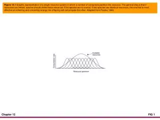
Figure 12.1 Graphic representation of a single resource system in which a number of consumers partition the resource. The general idea is that if resources are limited, species should divide those resources if the species are to coexist. If two species use identical resources, the one that is most effective at collecting and converting energy into offspring will outcompete the other. Adapted from Pianka, 1988.
Figure 12.2 A generalized food web for an eastern North American pond showing the bullfrog (Lithobates catesbeianus) as the focal point. Arrows denote direction of energy flow, i.e., consumption. The inset (lower right) shows the general pattern of energy flow through communities. Adapted from Bury and Whelan, 1984.
Figure 12.3 Relative abundance of skink assemblages in three habitats at Sakaerat, Thailand. Eleven species occur in the evergreen forest, and subsets occur in the deciduous forest and agriculture areas. The species are ranked in order of decreasing abundance for the evergreen forest assemblage, and that order is retained for the two other assemblages. Skink abundance is unequal between habitats; skinks comprise 53%, 43%, and 4% of the total lizards for the three habitats, respectively. Data from Inger and Colwell, 1977.
Figure 12.4 Abundance of lizards at Brazilian Cerrado site, based on pitfall trapping. Genera from left to right: Cnemidophorus, Tropidurus, Vanzosaura, Micrablepharus, Ameiva, Gymnodactylus, Colobosaura, Mabuya, Mabuya, Briba, Anolis, and Tupinambis. Adapted from Vitt et al., 2007b.
Figure 12.5 Relationship between structural microhabitat variables and lizard species in the Cerrado based on a Canonical Correspondence Analysis, which ordinates lizard species along two multivariate axes. Species are the same as in Figure 12.4. Adapted from Vitt et al., 2007b.
Figure 12.6 Relationship between island size and species richness of the Sphaerodactylus (squares) and lizard (circles) faunas in the West Indies. Dashed line depicts the islands with only a single species. Data from Schwartz and Henderson, 1991.
Figure 12.7 Two spadefoot toads that can produce carnivorous tadpoles in response to the presence of fairy shrimp. Left, Spea multiplicata; right, S. bombifrons.
Figure 12.8 Character change in two species of Spea. In the top panel, S. multiplicata responds to the presence of S. bombifrons by producing fewer of the carnivore phenotypes, indicating that character displacement has occurred. In the lower panel, production of carnivores by S. bombifrons is facultatively enhanced by presence of S. multiplicata, and production of carnivores by S. multiplicata is facultatively suppressed by presence of S. bombifrons. Adapted from Pfennig et al., 2000.
Figure 12.9 Alternative mechanisms influencing production of carnivore versus omnivore morphs in Spea multiplicata in response to presence of S. bombifrons. Tadpoles that ingest fairy shrimp have a probability p of producing carnivores and a probability 1-p of producing omnivores (the default morph). S. bombifrons modifies the morphological switch in S. multiplicata by character displacement (A) or phenotypic plasticity (B). In (A), S. multiplicata tadpoles have a fixed response to S. bombifrons, but the response differs in areas where they don't occur together (allopatric, Pall) and where they do occur together (sympatry, Psym). Phenotypic plasticity results from the ability of S. multiplicata to be influenced by S. bombifrons in its response to shrimp chemical cues (i.e., interference competition) or ability to detect shrimp chemical cues (B. ii., exploitative competition). Adapted from Pfennig and Murphy, 2000.
Figure 12.10 Graphic representation showing differences between long-term and far-flung studies in animal ecology. Abbreviation: t = time. Adapted from Cody, 1996.
Figure 12.11 The agamid lizard Moloch horridus (left) of Australia is an ecological equivalent of the iguanid lizard Phrynosoma platyrhinos of North America. Both species are ant specialists in arid habitats. Photos by E. R. Pianka (left) and L. J. Vitt (right).
Figure 12.12 Annual variation in proportional representation of three turtle species in Michigan, based on capture–recapture studies. Adapted from Congdon and Gibbons, 1996.
Figure 12.13 Incidence matrix showing occurrence of 14 amphibian species across 36 ponds on the E. S. George reserve in Michigan. Blackened squares indicate that a species was present at a particular pond at least once during the 7-year study. Ponds are rank-ordered in relation to two environmental variables: increasing canopy cover and increasing area and hydroperiod. Adapted from Werner et al., 2007.
Figure 12.14 Annual changes in amphibian species richness for all ponds combined at the E. S. George Reserve in Michigan. Three ponds lost fish in fall of 1998 or in 1999. Species richness of these ponds is indicated by closed circles. Prior to loss of fish, these three ponds had amphibian species richness similar to that of ponds containing fish. Amphibian species richness increased dramatically following loss of fish. Adapted from Werner et al., 2007.
Figure 12.15 Ecomorphs of Anolis lizards in the Caribbean. α and β indicate different (independent) clades of anoles. Adapted from Williams, 1983.
Figure 12.16 Patterns of community evolution in Jamaican (left) and Puerto Rican (right) Anolis lizards. Progression downward through communities within islands shows the evolution of anole ecomorphs. Comparison across islands (e.g., compare four-species communities) shows that evolution of ecomorphs in Anolis living on different islands is convergent. Adapted from Losos, 1992.
Figure 12.17 Diagram of the major events that occurred during the evolutionary history of squamate reptiles that affect their present-day ecology. Streptostyly, the hanging-jaw mechanisms set squamates apart from their sister taxon Rhynchocephalia. This allowed greater jaw mobility. The switch from lingual prehension (ancestral) to jaw prehension in scleroglossans freed the tongue for other uses. In gekkotans, the tongue was used as a windshield wiper for the spectacle over the eye and to clean the lips, but they also developed an effective nasal olfactory system. In autarchoglossans, the tongue and vomeronasal organ provided an effective chemosensory system, allowing prey discrimination among other things. Other correlates include differences in foraging mode, behavior, and physiology (see also Chapters 6-11). Adapted from Vitt et al., 2003.
Figure 12.18 Differences in activity periods (top) and microhabitat use (bottom) exist between the three major squamate lizard clades. Adapted from Vitt et al., 2003.
Figure 12.19 Major dietary shifts occurred during the evolutionary history of squamate lizards. Each numbered divergence point represents a statistically significant dietary shift, and taken together, these six divergence points account for 80% of the variation among species in diets. Adapted from Vitt and Pianka, 2005, 2007.
Figure 12.20 Changes in the proportional representation of three clades of colubrid snake species in communities across a latitudinal gradient from northern Central America to southern South America. The points at each north–south location represent specific snake communities. For example, the first set of points represents the snake fauna at Los Tuxtlas, Mexico, where 36% are Central American xenodontines (circle), 11% are South American xenodontines (triangle), and 53% are colubrines (square). Numbers along the x-axis represent rank order of localities along the north–south gradient. Values on the x-axis do not correspond to the original categories used by Cadle and Greene (1993). Ranking by latitude changed the positions of the five sets of points at the southern latitude end of the graph. The dashed line separates Central American from South American localities. Adapted from Cadle and Greene, 1993.
Figure 12.21 Three possible outcomes of using niche modeling to examine distributions of closely related species across environmental gradients. (A) No overlap in predicted distributions, (B) both species occurring in the area of predicted overlap, and (C) one of the species occurring in the area of predicted overlap. Adapted from Costa et al., 2007.
Figure 12.22 East–west gradient in six environmental variables used to model fundamental niches of six species pairs of amphibians and reptiles. Variables shown are (a) altitude, (b) mean annual precipitation, (c) precipitation of the driest quarter, (d) precipitation seasonality, (e) minimum temperature of the coldest month, and (f) temperature seasonality. Temperature variables are in °C, precipitation variables are in mm, and altitude is in m. Adapted from Costa et al., 2008.
Figure 12.23 Distribution maps for six species pairs of amphibians and reptiles, based on niche modeling. Open circles indicate species with western distributions; closed circles represent species with eastern distributions. Yellow indicates distribution of the western species within Oklahoma, blue indicates distribution of the eastern species within Oklahoma, and red indicates an overlap zone, all based on niche modeling. Adapted from Costa et al., 2008.