Download
1 / 18
180 likes | 339 Views
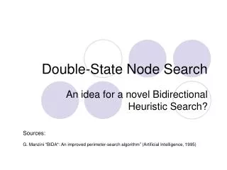
Double-State Node Search. An idea for a novel Bidirectional Heuristic Search?. Sources: G. Manzini “BIDA*: An improved perimeter-search algorithm” (Artificial Intelligence, 1995). Motivations & Objective. In problem solving we know the target, we should make the best use of it!

E N D
Double-State Node Search An idea for a novel Bidirectional Heuristic Search? Sources: G. Manzini “BIDA*: An improved perimeter-search algorithm” (Artificial Intelligence, 1995)
Motivations & Objective • In problem solving we know the target, we should make the best use of it! • Bidirectional Heuristic Search has not been really successfull, yet: only with the implementation of problem-specific techniques bidirectional algorithms performed better than Unidirectional ones. • The problem of Bidirectional Search is that it is complicated to check the optimality of its solutions. • Our objective is to propose a much simpler and “hopefully” effective approach to Bidirectional Search, by completely changing its perspective.
Outline of the talk • Introduction to admissible blind search: • unidirectional and bidirectional • Introduction to admissible heuristic search: • Unidirectional • Best-First Search: A* • Linear Space Search: IDA*, DFBnB • Bidirectional (see referenced papers for deeper analysis!) • Classic front-to-end bidirectional search: BHPA, BS* • The problem of classic bidirectional search • Front-to-front bidirectional search: BIDA* & perimeter search • A successful bidirectional search: differences and BAI • An alternative approach: “Double-state node search” • The idea & some preliminary results
Unidirectional optimal blind search • Unidirectional (breadth first) spatial cost: O(bd) time cost: O(bd) GOAL
Bidirectional optimal blind search • Bidirectional (breadth first) spatial cost: O(bd/2) time cost: O(bd/2) GOAL X0
Unidirectional Heuristic SearchBest-First Search • Best-First Search uses two lists: OPEN (frontier) and a CLOSED (expanded nodes) • It always expands from the frontier the most promising node, e.g. the node n with the smallest f(n) • Uniform-Cost Search: f(n) = g(n) • Greedy Search: f(n) = h(n) • A*: f(n) = g(n) + h(n) • Weighted A*: f(n) = (1-w) * g(n) + w * h(n) • A* properties: • given an admissible heuristic h, A* is optimal and optimally efficient • A* has exponential time and memory costs.
Unidirectional Heuristic SearchLinear Space Search • IDA*: depth-first iterative deepening search • At each iteration IDA* completes a depth-first search of all the nodes that have a f(n) = g(n) + h(n) threshold • The threshold is updated at each iteration to the value of the lowest cost node pruned during the previous iteration • IDA* runs with linear spatial cost and does not have the overhead of managing the OPEN and CLOSED lists • Major problem: if the operator cost is not constant the time cost could be up to O(b2d) • DFBnB: depth-first search branch&bound • Depth-first search that keeps track of the best solution (s) so far • Prune all the branches with cost equal or greater than s • For finite search trees (e.g. TSP) is better than IDA*
n’ hf(n’) s t hb(n’’) n’’ front-to-end heuristics Bidirectional Heuristic SearchBHPA: the first algorithm (Pohl ‘71) • Bi-directional Heuristic Path Algo. (BHPA) is made of 2 “simultaneous” A* searches in opposite directions using two heuristics: one forward, hf , and one backward, hb • At each expansion the direction is chosen following the cardinality criterion: • if |OPENf| < |OPENb| thendir = felsedir = b • The algorithm terminates when: The best complete solution found so far is not larger that the maximum best fd (max of both directions) in the frontier
Bidirectional Heuristic SearchBS* (Kwa ‘89) • BS* is logically identical to BHPA but incorporates the termination condition implicitly, by removing (trimming) and not placing (screening) the nodes with fd ≥ Lmin • BS* terminates when OPENf or OPENb is empty • BS* uses two additional techniques: • nipping: a node chosen for expansion that is in CLOSED in the opposite direction can be put into CLOSED without expansion • pruning: after nipping all the descendants of the node that are in OPEN in the opposite direction can be removed
The problem of front-to-end search • A* performs as or better than BHPA and BS*! Why? • #(BHPA) ≈ 2(#A*) and not #(BHPA) ≈ √#(A*) as suggested by blind search theory • The Missile Metaphor? • The two searches pass each other without touching, like two missiles? • This conjecture (Pohl, Nilsson) is wrong! • The two searches go through each other! The problem is guaranteeing the optimality.
The problem of front-to-end search (2) • The problem of bidirectional search using front-to-end heuristics is that of guaranteeing the optimality of the encountered solutions not that of making the two searches encounter (thus finding a solution) • BS* on the 15-puzzle (Kaindl, ‘93) • BS* finds the first solution after 7.2% of total node generation • The first solution is only 6.3% worse that optimal • The optimal solution is found after 22.4% of node generation (77.6% of search is devoted to proving its optimality!) • For this reason BS* is one the of the best -admissible algorithms
Front-to-front perimeter search(BIDA*, Manzini ‘95) • BIDA* is based on two different steps: • a breadth-first search generates the nodes around the target and stores all the nodes of the frontier (perimeter) with their h* value (k in figure below) • IDA* forward search using front-to-front evaluations • front-to-front evaluations are computed as: • unnecessary nodes can be removed from the frontier to speed up computation
Perimeter search evaluation • Perimeter search is efficient only under two conditions: • when IDA* is feasible (operators with constant cost) • when the depth of the optimal solution is small • Good results with 15-puzzle, poor performances with path finding 2000x2000 path finding: avg. d = ca. 3000, a perimeter of 50, covers only 1,7% 15-puzzle: avg. d = 52,7 (a perimeter of 15 covers nearly 30% of the distance)
Differences: a better front-to-end search • During search, A* (or IDA*) discovers “differences” between g(n) and the h(n) in the opposite direction. • In this example: fmin2 provides the minimum f value estimated in the backward search. Diff2 provides the backward heuristic error on node A.
Performance of the“differences approach” • 15-puzzle: • backward search with A* and forward with IDA* • Very good performances using IDA*+differences with a lot of “tricks”: transposition tables, nipping (like BS*), dynamic choice of IDA* direction (probing). • 2000x2000 path-finding: • Differences + A*A*, the impact is modest. The success of the approach relies on the problem and IDA* “tricks”. 15-puzzle Path-finding
1 2 3 1 2 3 1 2 3 4 4 8 8 8 5 5 5 1 2 3 1 1 2 2 3 3 1 2 3 4 7 6 7 6 7 6 4 5 8 4 5 5 4 5 6 7 8 6 4 7 8 7 6 6 7 8 1 2 3 4 8 5 7 6 Double-state node search: insight • The idea: instead of “hoping” that two opposite searches somehow meet eachother and that the sum of the two paths is optimal: “unidirectionally search the shortest path to make the start and the target equal” (example below) • We don’t know the target, but we have an admissible heuristic: the manhattan difference between the two states (like front-to-front evaluation). S T A R T G O A L =
a z z1 z2 zb z1 z2 zb z1 z2 zb a1 a1 a1 a2 a2 a2 ab ab ab Double-state node search: basics • For optimality, the heuristic must underestimate how many moves we still have to do to make the two states equal. • The nodes of the search tree will contain two states, one “closer” to the start and one “closer” to the target. • The two states will not be stored within the node, but simply referenced by the node using a pointer. • At each expansion the algorithm generates max. b2 nodes, pointing to max. 2b different states. a1 a2 ab z1 z2 zb
a z b2 d/2 Double-state node search: advantages • Simple termination policy: with an admissible heuristic, any A* implementation will find the optimal solution at first! • Any unidirectional admissible algorithm can be used, so that the approach does not rely on the problem’s properties. • Any relative-error-heuristic (as in all real problems) will tend to have a smaller error than in classic front-to-end search, since h* will be smaller on average. • Memory saving! Using plain A*: the number of nodes expanded will be O(b2*d/2) = O(bd), as unidirectional search (hence the number of pointers will be 2*O(bd)), but the number of states stored will only be approx. O(2bd/2) With A* algorithm: #nodes: (b2)d/2=bd #states: (2b)d/2 nodes affect time cost and states affect mem