Download
1 / 19
190 likes | 447 Views
iSWWS-2013@NCU, Taiwan. Group A. CME acceleration / deceleration. Tomoya Iju (Nagoya University, Japan) Nai Hwa Chen (National Central University, Taiwan). Group Presentation. 1. Our Work. Understanding the rapid acceleration and subsequent deceleration of CME.

E N D
iSWWS-2013@NCU, Taiwan Group A. CME acceleration /deceleration Tomoya Iju (Nagoya University, Japan) Nai Hwa Chen (National Central University, Taiwan) Group Presentation
1. Our Work • Understanding the rapid acceleration and subsequent deceleration of CME. • We attempt to draw a complete height-time and distance-velocity profiles of CME from the lower solar corona to the Earth. • In this work, we use data of Wind/WAVES radio experiment, SOHO/LASCO coronagraph, interplanetary scintillation (IPS), STEREO/HI heliospheric camera, and in-situ measurements. • We search the CME event detected by all of the above methods, and then find an event.
Feb. 15, 2011 CME (X2.2 flare in AR 11158) SOHO/LASCO C2 and SDO/AIA
Interplanetary Part of Feb. 15, 2011 CME 02/15, 03:54 02/15, 15:29 02/16, 20:09 STEREO-A/COR2, HI-1, and HI-2
Feb. 15, 2011 CME associated type-II and type-III radio burst X2.2 flare occur at 01:55 Wind/WAVES Type-II burst
IPS observation allow us to probe into the inner heliosphere with a cadence of 24 hours. 2.CME Observation using Interplanetary Scintillation (IPS) ↑Solar Wind Imaging Facility (SWIFT) in Toyokawa city ↑ KISO Radio Telescope
3. Solar Wind Disturbance Factor ‘g-value’ • For each radio source, the g-value is defined as the ratio of observed index ‘m’ to mean value ’my’: quiet:g~1 disturbed:g>1
The approximation that a large fraction of scintillation is given by the radio wave scattering at the P-point on a line-of-sight (Hewish, Scott, and Wills, 1964). A sky-map of enhanced g-values, ‘g-map’, provides information on the spatial distribution of CME between 0.2 and 1 AU.
4. Identification of ICME Detected by LASCO, IPS, and in-situ Observations • We assumed that • (1) An CME caused a disturbance event day • (2) An CME lie in a region of enhanced g-values in the g-map • The criterion for observation date SOHO/LASCO → IPS → In-situ observation (ACE, etc) ( DED ) In-situ CME detection
Reference distances R1,2and velocities V1,2 5. Calculation of CME Velocity in IPS SOHO-IPS: Here, tSOHOis CME appearance time, dSOHO is Minimum radius of LASCOC2 F.O.V, P-point distance dIPSand observation time tIPS for a g≧1.5 radio source, tACE is CME detection time at ACE, and dACE~1AU IPS-ACE:
6. Estimation of CME Velocity from Type-II Radio Burst • 5 fold Saito model (1970, 1977). • Using this relation, we can estimate the associated height and velocity from the radio frequency measurements.
7. Estimation of CME Velocity from in-situ Observations • We identify the near-Earth part of Feb. 15, 2011 CME ourselves using data of solar wind charge states obtained by the ACE/SWICS, and criteria of near-Earth CME identification, i.e., the abruptly increase of charge states for Fe and of O7/O6 ratio during the passing of a CME (Richardson and Cane, 2010). • We define that the velocity of near-Earth CME is the average flow speed during the charge stateenhancement.
9. Question • We can fit not only data points for the LASCO, IPS, and in-situ observations but also those for the type-II radio burst by a straight line in a logarithmic height-time plot. • Why different slopes of lines for the type-II radio burst and the other observations? • Whether kilometric type-II burst reflects dynamics of CME or not? • We confirm that the CME velocity derived from the IPS, HI-1 and 2 shows the similar value in the range of ~400km/s to ~600km/s.
10. Discussion • the CME velocity derived from the IPS, HI-1 and 2 indicates that the Feb. 15, 2011 CME rapidly decelerate by the interaction with the solar wind. • The starting timing of type II radio burst is 9 minutes before the CMEs front shown in LASCO C2. the X class flare occurs at 01:55. • We speculate that the shock front of CME generating the type II burst is in LASCO C2 FOV before appearance of CME’s leading edge. • We need further study for the relationship between CME and type-II burst.
Top right: Fast CME (V-Vbg) > 500 km/s Bottom right: Moderate CME 0 km/s ≦ (V-Vbg) ≦500 km/s Bottom left: Slow CME 0 km/s < (V-Vbg)
Conclusion • We draw a height-time and distance-velocity profiles of Feb. 15, 2011 CME from the solar corona to the Earth. • The distance-velocity profile derived from the type-II radio burst shows the rapid acceleration, and the CME velocity derived from the IPS, HI-1 and 2 exhibits the similar value in the range of ~400km/s to ~600km/s. This indicate rapid decelerate of CME by the interaction with the solar wind.