Download
1 / 18
180 likes | 255 Views
Learn to derive the equations of motion for simple and compound pendulums, including natural frequency calculations. Understand the kinetic and potential energy involved with no external excitation or damping. Gain insights into Lagrange's equations for mechanical systems.

E N D
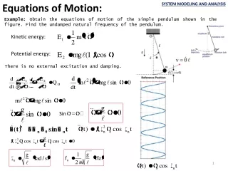
Equations of Motion: SYSTEM MODELING AND ANALYSIS Example: Obtain the equations of motion of the simple pendulum shown in the figure. Find the undamped natural frequency of the pendulum. Kinetic energy: Potential energy: There is no external excitation and damping. Sin≈
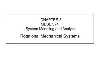
SYSTEM MODELING AND ANALYSIS O m, L, IO L1 g G L θ Example: Obtain the equations of motion of the compound pendulum shown in the figure. Find the undamped natural frequency. Kinetic energy: Potential energy: Where IO is the mass moment of inertia about point O. For small angular displacements sin θθ
SYSTEM MODELING AND ANALYSIS L1=0.170299 m Material: Plain carbon steel
SYSTEM MODELING AND ANALYSIS 0.92 (s) 1.88 (s)
SYSTEM MODELING AND ANALYSIS Example: Obtain the equations of motion of the mechanical system shown in the figure. Yücel Ercan, İleri Dinamik 2014. M1 Solution: System has two degree of freedom, namely θ and x. x θ Bob Pendulum rod Tranlational mass Kinetic energy: Potential energy: Virtual work:
SYSTEM MODELING AND ANALYSIS Lagrange’s equation for θ: Kinetic energy: Potential energy: Virtual work:
Lagrange’s equation for x: (For constant M) In matrix form;
SYSTEM MODELING AND ANALYSIS Example: Obtain the equations of motion of the mechanical system shown in the figure. Solution: (Kinetic energy of the beam is zero due to its negligible mass) x Lagrange’s equation for θ:
SYSTEM MODELING AND ANALYSIS Lagrange’s equation for x: In matrix form;
SYSTEM MODELING AND ANALYSIS Example: Obtain the equations of motion of the mechanical system shown in the figure. G Inputs: f, T, x4 Outputs Potential energy of pendulum is neglected
SYSTEM MODELING AND ANALYSIS In matrix form:
(Free vibration) Eigenvalue equation EIGENVALUE EQUATION Eigenvalue equation:
Eigenvalue equation: m=0.85 kg, L =0.24 m, k=1200 N/m, c=20 Ns/m Matlab code: This value is different in the original presentation clc;clear m=0.85;l=0.24;k=1200;c=20; M=[m*l^2/8,0;0,3*m/4]; %Mass matrix C=[27*c*l^2/16,-9*c*l/4;-9*c*l/4,6*c]; %Damping matrix K=[9*k*l^2/8,-3*k*l/2;-3*k*l/2,4*k]; %Stiffness matrix syms s; %Symbolic variable definition mtr=M*s^2+C*s+K; p=solve(det(mtr)) %Eigenvalues of the system vpa(p,5) Eigenvalues: -34.163+39.572i, -34.163-39.572i, -44.572, -393.02
Eigenvalues: -34.163+39.572i, -34.163-39.572i, -44.572, -393.02 θh(t) = C1e(-34.163+39.572i)t + C2e(-34.163-39.572i)t + A2e-44.572t + A3e-393.02t (Complex coefficients)
p=-σ+iω iω ω0 φ -σ Real eigenvalues correspond to an exponential time response Complex eigenvalues correspond to an exponential-harmonic time response Form of the free vibration response: A1, φ1, A2 and A3 can be calculated from initial conditions The output reaches to zero as time t goes infinity. If the real parts of all eigenvalues are negative than the system is stable. rad/s For the root -44.572 Δt=0.0071, t∞=0.141 p=-σ For the root -393.02 Δt=0.0008 , t∞=0.016 Use smallest t and largest t For the system Δt=0.0008 , t∞=0.1839
x(t) x(t) 1 0.5 5 0.2 3 ξ=0.1 t t