Download
1 / 46
461 likes | 575 Views
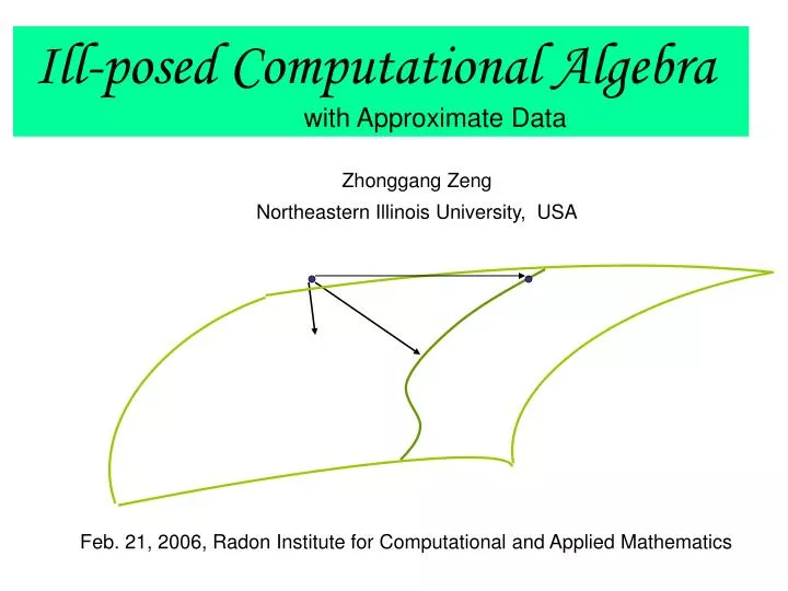
Ill-posed Computational Algebra with Approximate Data. Zhonggang Zeng Northeastern Illinois University, USA. Feb. 21, 2006, Radon Institute for Computational and Applied Mathematics. = 4 nullity = 2. Rank. null space. basis.

E N D
Ill-posed Computational Algebra with Approximate Data Zhonggang Zeng Northeastern Illinois University, USA Feb. 21, 2006, Radon Institute for Computational and Applied Mathematics
= 4 nullity = 2 Rank null space basis Example: Matrix rank and nulspace + eE = 6 nullity = 0 2
Ill-posed problems are common in applications • image restoration - deconvolution • IVP for stiction damped oscillator - inverse heat conduction • some optimal control problems - electromagnetic inverse scatering • air-sea heat fluxes estimation - the Cauchy prob. for Laplace eq. • … … • A well-posed problem: (Hadamard, 1923) • the solution satisfies • existence • uniqueness • continuity w.r.t data An ill-posed problem is infinitely sensitive to perturbation tiny perturbation huge error 3
- Multiple roots of polynomials - Polynomial GCD - Factorization of multivariate polynomials - The Jordan Canonical Form - Multiplicity structure/zeros of polynomial systems - Matrix rank Ill-posed problems are common in algebraic computing 4
Problem: Polynomial factorization (E. Kaltofen, Challenges of symbolic computation, 2000) Exact factorization no longer exists under perturbation Can someone recover the factorization when the polynomial is perturbed? 5
Problem: polynomial root-finding Exact roots 1.072753787571903102973345215911852872073… 0.422344648788787166815198898160900915499… 0.422344648788787166815198898160900915499… 2.603418941910394555618569229522806448999… 2.603418941910394555618569229522806448999 … 2.603418941910394555618569229522806448999 … 1.710524183747873288503605282346269140403… 1.710524183747873288503605282346269140403… 1.710524183747873288503605282346269140403… 1.710524183747873288503605282346269140403… Inexact coefficients 2372413541474339676910695241133745439996376 -21727618192764014977087878553429208549790220 83017972998760481224804578100165918125988254 -175233447692680232287736669617034667590560780 228740383018936986749432151287201460989730170 -194824889329268365617381244488160676107856140 110500081573983216042103084234600451650439720 -41455438401474709440879035174998852213892159 9890516368573661313659709437834514939863439 -1359954781944210276988875203332838814941903 82074319378143992298461706302713313023249 “attainable” roots 1.072753787571903102973345215911852872073… 0.422344648788787166815198898160900915499… 0.422344648788787166815198898160900915499… 2.603418941910394555618569229522806448999… 2.603418941910394555618569229522806448999 … 2.603418941910394555618569229522806448999 … 1.710524183747873288503605282346269140403… 1.710524183747873288503605282346269140403… 1.710524183747873288503605282346269140403… 1.710524183747873288503605282346269140403… 9 3 5 5 Exact coefficients 2372413541474339676910695241133745439996376 -21727618192764014977087878553429208549790220 83017972998760481224804578100165918125988254 -175233447692680232287736669617034667590560789 228740383018936986749432151287201460989730173 -194824889329268365617381244488160676107856145 110500081573983216042103084234600451650439725 -41455438401474709440879035174998852213892159 9890516368573661313659709437834514939863439 -1359954781944210276988875203332838814941903 82074319378143992298461706302713313023249 -6-
Special case: Maple takes 2 hours On a similar 8x8 matrix, Maple and Mathematica run out of memory Question: can we compute the JCF using approximate data? Example: JCF computation 7
Question: Can we find the JCF approximately when Lancaster matrix derived from stability problem 8
310 0 0 0 0 0 0 0 0 0 0 0 0 0 0 0 0 0 0 0 0310 0 0 0 0 0 0 0 0 0 0 0 0 0 0 0 0 0 0 0 0310 0 0 0 0 0 0 0 0 0 0 0 0 0 0 0 0 0 0 0 0310 0 0 0 0 0 0 0 0 0 0 0 0 0 0 0 0 0 0 0 0310 0 0 0 0 0 0 0 0 0 0 0 0 0 0 0 0 0 0 0 0310 0 0 0 0 0 0 0 0 0 0 0 0 0 0 0 0 0 0 0 0310 0 0 0 0 0 0 0 0 0 0 0 0 0 0 0 0 0 0 0 0310 0 0 0 0 0 0 0 0 0 0 0 0 0 0 0 0 0 0 0 0310 0 0 0 0 0 0 0 0 0 0 0 0 0 0 0 0 0 0 0 030 0 0 0 0 0 0 0 0 0 0 0 0 0 0 0 0 0 0 0 0 0310 0 0 0 0 0 0 0 0 0 0 0 0 0 0 0 0 0 0 0 0310 0 0 0 0 0 0 0 0 0 0 0 0 0 0 0 0 0 0 0 0310 0 0 0 0 0 0 0 0 0 0 0 0 0 0 0 0 0 0 0 0310 0 0 0 0 0 0 0 0 0 0 0 0 0 0 0 0 0 0 0 0310 0 0 0 0 0 0 0 0 0 0 0 0 0 0 0 0 0 0 0 0310 0 0 0 0 0 0 0 0 0 0 0 0 0 0 0 0 0 0 0 030 0 0 0 0 0 0 0 0 0 0 0 0 0 0 0 0 0 0 0 0 0310 0 0 0 0 0 0 0 0 0 0 0 0 0 0 0 0 0 0 0 0310 0 0 0 0 0 0 0 0 0 0 0 0 0 0 0 0 0 0 0 0310 0 0 0 0 0 0 0 0 0 0 0 0 0 0 0 0 0 0 0 031 0 0 0 0 0 0 0 0 0 0 0 0 0 0 0 0 0 0 0 0 03 JCF Problem: Jordan Canonical Form (JCF) 0 10 3 0 -1 -1 -4 0 0 -5 -5 0 1 0 0 -1 0 -5 -1 0 -3 -1 0 5 9 -1 3 -2 -1 1 1 -2 -2 1 -1 1 1 2 -1 -1 1 0 -1 1 3 1 7 2 -2 -11 1 0 6 -4 -3 6 0 5 -1 0 -3 -2 -1 0 0 0 -1 1 5 2 3 1 -1 0 0 0 0 0 -1 0 1 2 0 0 1 0 -1 1 -4 -2 -9 -2 6 19 -2 0 -8 8 6 -8 1 -7 1 -2 4 4 2 0 0 -1 0 -1 1 -1 1 2 1 1 0 0 0 0 0 0 1 0 0 0 0 0 0 0 0 1 9 -2 4 -3 3 3 1 -2 -2 1 0 1 2 1 -1 -1 1 0 -1 0 1 0 1 0 0 -2 0 3 4 0 0 3 0 2 0 0 -1 0 0 0 0 0 1 -4 -2 0 1 4 1 0 3 5 4 0 -2 0 0 1 0 3 1 0 1 1 -1 1 -2 1 -1 3 -1 -1 -3 3 0 -3 0 -2 -1 0 1 0 0 0 0 0 5 2 6 2 -3 -16 1 0 12 -5 -1 12 0 9 -1 0 -5 -3 -2 0 0 0 -1 4 0 1 -2 -4 -1 0 0 -5 -4 3 4 0 -1 -2 0 -3 -1 0 -1 -2 1 0 1 0 0 -2 0 0 2 0 0 2 3 2 0 0 -1 0 0 0 0 0 0 -1 4 -3 3 -1 1 1 0 0 0 0 -2 3 3 1 0 0 0 0 0 1 0 2 12 -1 2 -7 0 0 2 -4 -3 2 -3 2 4 6 -1 -2 0 0 -1 3 -4 -1 -5 -2 2 12 -1 0 -7 4 3 -7 0 -6 1 3 4 2 1 0 0 0 0 11 8 1 -2 -12 -3 0 6 -9 -8 6 1 5 0 -1 0 -7 -2 0 -3 -1 -2 0 7 -2 5 1 -1 1 -2 0 0 -2 0 -1 1 1 0 4 3 -1 -1 0 3 2 6 2 -2 -7 1 0 2 -5 -4 2 -2 2 0 3 -1 -3 1 2 0 2 5 -12 -10 2 -3 1 5 -1 0 6 6 0 0 0 -2 -1 0 6 0 3 5 0 4 -9 0 1 0 1 4 -1 0 4 4 0 -4 0 0 4 0 4 0 1 6 4 2 0 2 0 0 -3 0 0 3 0 0 3 0 3 0 0 -2 0 0 0 0 3 9
An approximate zero x0is an exact solution to Problem: Multiplicity structure of a polynomial system A zero x* can only be approximate, even if P is exact (Abel’s Impossibility Theorem) x0 degrades to a simple zero, even if x* is multiple Can we recover the lost multiplicity structure? 10
Solution P P Data P Challenge in solving ill-posed problems: Can we recover the lost solution when data is inexact? P:Data Solution 11
Wilkinson’s Turing Award(1970): However: Ill-posed problems are infinitely sensitive to data perturbation A numerical algorithm seeks the exact solution of a nearby problem If the answer is highly sensitive to perturbations, you have probably asked the wrong question. Maxims about numerical mathematics, computers, science and life, L. N. Trefethen. SIAM News Conclusion: Numerical computation is incompatible with ill-posed problems. Solution: Ask the right question. 12
(Distance to singular matrices) Trivia quiz: Is the following matrix nonsingular? (matrix derived from polynomial division by x+10 ) Answer: It is nonsingular in pure math. Not so in Numerical Analysis. 13
B A i.e. the worst rank of nearby matrices with I.e. the nulspace of the nearest matrix with that rank Rank problem: Ask the right question • nearness • max-nullity • mini-distance 14
= 4 nullity = 2 = 4 nullityq = 2 After reformulating the rank: Rank Rankq null space basis + eE = 6 nullity = 0 + eE = 4 nullityq = 2 Ill-posedness is removed successfully. 15
Computing approximate rank/nullspace: General purpose: Singular value decomposition (SVD) Low-nullity and low-rank cases: Recursive Inverse iteration/deflation (T.Y. Li & Z. Zeng, SIMAX 2005) Software package RankRev available 16
For given polynomials f and g, find u, v, w such that which is an important application problem in its own right. Applications: Robotics, computer vision, image restoration, control theory, system identification, canonical transformation, mechanical geometry theorem proving, hybrid rational function approximation … … Problem: Polynomial GCD 17
If then nulspace The Sylvester Resultant matrix is approximately rank-deficient The question: How to determine the GCD structure At heart of the GCD-finding is calculating rank and nulspace with an approximate matrix 18
-- space of polynomial pairs • nearness • max-degree • mini-distance i.e. the max degree of nearby polyn’s with I.e. the GCD of the nearest polyn pair with that degree 19
-- space of polynomial pairs perturbed polynomial pair original polynomial pair computed polynomial pair manifold Minimize A two staged approach: Determine the GCD structure (or manifold) Reformulate – solve a least squares problem well-posed, and even well conditioned 20 --- a least squares problem
The strategy: Reformulate a well-posed problem Given Set up a system for Or, in vector form where and minimize and the GCD degree k 21
Its Jacobian: In other words: if the AGCD degree k is correct, then is a regular, well-posed problem! Theorem: The Jacobian is of full rank if v and w are co-prime 22
S2(f,g) S1(f,g) = QR QR by formulating and the Gauss-Newton iteration For univariate polynomials : Stage I: determine the GCD degree until finding the first rank-deficient Sylvester submatrix Stage II: determine the GCD factors ( u, v, w ) 23
Max-degree k := k-1 k := k-1 Is GCD of degree k possible? no no probably Refine with G-N Iteration Successful? yes Min-distance nearness Output GCD Start: k = n Univariate AGCD algorithm 24
Software packages Corless-Watt-Zhi Gao-Kaltofen-May-Yang-Zhi Kaltofen-Yang-Zhi etc Zeng: uvGCD – univariate GCD computation mvGCD – multivariate GCD computation 25
distinct roots: u0(x) = [(x-1)4(x-2) 2] [(x-1)(x-2)(x-3)] * * * u1(x) = [(x-1)3(x-2) ] [(x-1)(x-2)] * * u2(x) = [(x-1)2] [(x-1)(x-2)] * * u3(x) = [(x-1)] [(x-1)] * u4(x) = [1] [(x-1)] * ----------------------------------------- multiplicities 5 3 1 Identifying the multiplicity structure p(x)= (x-1)5(x-2) 3(x-3) = [(x-1)4(x-2) 2] [(x-1)(x-2)(x-3)] p’(x)= [(x-1)4(x-2) 2][ (x-1)(x-2)+5(x -2)(x -3)+3(x -1)(x -3)] GCD(p,p’) = [(x-1)4(x-2) 2] u0 = p um =GCD(um-1, um-1’) 26
the key with vj’s being squarefree Output : f = v1 v2 … vk - The multiplicity structure A squarefree factorization of f: u0 =f for j = 0, 1, … while deg(uj) > 0 do uj+1 = GCD(uj, uj’) vj+1 = uj/uj+1 end do - The number of distinct roots: m = deg(v1) - Roots of vj’s are initial approximation to the roots of f 27
For the ill-posed multiple root problem with inexact data The key: Remove the ill-posedness by reformulating the problem Original problem: calculating the roots Reformulated problem: finding the nearest polynomial on a proper pejorative manifold -- A constraint minimization 28
(m<n) (degree) n m (number of distinct roots) To calculate roots of p(x)= xn + a1xn-1+...+an-1 x + an Let ( x - z1 )l1( x - z2)l2 ... ( x - zm)lm = xn + g1( z1, ..., zm )xn-1+...+gn-1( z1, ..., zm) x + gn( z1, ..., zm ) Then, p(x) = ( x - z1 )l1( x - z2)l2 ... ( x - zm)lm <==> g1( z1, ..., zm )=a1 g2( z1, ..., zm)=a2 ... ... ... gn( z1, ..., zm )=an I.e. An over determined polynomial system G(z) = a 29
given polynomial b ~ q(x) a original polynomial Gl(z) = a ~ p b computed polynomial It is now a well-posed problem! 30
Stage II results: The backward error: 6.16 x 10⁻¹⁶ Computed roots multiplicities 1.000000000000000 20 1.999999999999997 15 3.000000000000011 10 3.999999999999985 5 For polynomial with (inexact ) coefficients in machine precision Stage I results: The backward error: 6.05 x 10⁻¹⁰ Computed roots multiplicities 1.000000000000353 20 2.000000000030904 15 3.000000000176196 10 4.000000000109542 5 Software: MultRoot, Zeng, ACM TOMS 2004 31
l 1 l 1 l l 1 l J = l 1 l l l l l l + + + + + + + + + + + + + + + + lI+S= l l l + + + 3 2 2 1 4 l Ferrer’s diagram 3 1 JCF computing: For a given matrix A find X, J: AX = XJ Segre characteristics: [3,2,2,1] find U, S, l AU = U(lI+S) Staircase form with Weyr characteristics: [4,3,1] 32
If the Weyr characteristics is known: find U, S, l AU = U(lI+S) leads to AU- U(lI+S) = 0 UHU – I = 0 for l, U, S (1) l l l l + + + + + + + + + + + + + + + + BHU = 0 lI+S= l l l + + + l with a staircase structure constraint Theorem: Solving system (1) for a least squares solution is well-posed! -- Eigenvalues are no longer flying! -- Gauss-Newton iteration converges locally 33
A two-stage strategy for computing JCF: Stage I: determine the Jordan structure and an initial approximation Stage II: Solve the reformulated least squares problem at each eigenvalue, subject to the structural constraint, using the Gauss-Newtion iteration. 34
Minimal polynomials: A rank/nulspace problem, again eigenvalue Segre characteristics l1 5 3 2 2 l2 3 3 1 l3 2 Let v be a coefficient vector of p1. Then for a random x 35
leads to p2(l), p3(l), … recursively Rank/nulspace leads to p1(l) (the 1st minimal polynomial) By a Hessenberg reduction, with A1 = A, and x being the first column of Q1, 36
Minimal polynomials Ill-posed root-finding with approximate data GCD Root-finding JCF Computing multiple roots of inexact polynomials, Z. Zeng, ISSAC 03 Rank-revealing 37
-- space of matrices perturbed matrix original matrix Max-defectiveness: on P Nearness: JCF of “nearest” matrix on P We can obtain an approximate JCF of Mini-distance: from P to manifold When matrix A is possibly approximate: Software AJCF is in testing stage 38
For a problem (data ----> solution) with data D0 minimize A two-stage strategy for removing ill-posedness: Stage I: determine the structureSof the desired solution this structure determines a pejorative manifold of data P = P-1(S) = {D | P(D) = S fits the structure } Stage II: formulate and solve a least squares problem by the Gauss-Newton iteration 39
The multiplicity structure of polynomial systems Intersection multiplicity = (algebraic geometry) • Dual spaceD(0,0) (I) spanned by Differential orders 6 depth = 6 5 4 3 2 1 0 breadth=2 What’s the multiplicity of (0,0)? Example: • Multiplicity = 12 • Hilbert function = {1,2,3,2,2,1,1,0,…} Multiplicity is not just a number!
Multiplicity = m Differential functionals Vanish on the ideal <p>, and span the dual space of <p> at x0 The dual space defines the multiplicity structure of the ideal at x0 For a univariate polynomial p(x) at zero x0: Duality approach (Lasker, Macaulay, Groebner): Multiplicity is the dimension of the dual space, spanned by the differential functionals that vanish on the ideal 41
A differential functional c of order a with The functional c is in the dual space if and only if Or, equivalently A rank/nulspace problem, again! For a polynomial system, or ideal at zero z 42
Multiplicity matrices and nullspaces 43
If the polynomial system is inexact, or if the system is exact, but the zero is approximate determining the multiplicity structure goes back to solving Ill-posed rank/nulspace problem with approximate data. • Algorithm: • for a = 1, 2, … do - construct matrix Sa - compute - if Wa = {0}, break • end do A reliable algorithm for calculating the multiplicity structure with approximate data Dayton & Zeng, ISSAC 2005 Bates, Peterson & Sommese, 2005 44
Conclusion - Ill-posed problems could be regularized as well posed least squares problems • Regularized ill-posed problems permit approximated data • Rank/nulspace determination is at the heart of solving ill-posed problems Software package PolynMat : RankRev uvGCD mvGCD MultRoot AJCF dMult