Download

1 / 77
770 likes | 978 Views
Optimal Design For Large-Scale Ill-posed Problems. Lior Horesh Joint work with E. Haber, L. Tenorio. IBM TJ Watson Research Center Large-Scale Inverse Problems and Uncertainty Quantification, Santa Fe, NM - May 2013. Introduction. Exposition - ill - posed Inverse problems.

E N D
Optimal Design For Large-Scale Ill-posed Problems LiorHoresh Joint work with E. Haber, L. Tenorio IBM TJ Watson Research Center Large-Scale Inverse Problems and Uncertainty Quantification, Santa Fe, NM - May 2013
Exposition - ill - posed Inverse problems • Aim: infer model • Given • Experimental design y • Measurements • Observation model • Ill - posedness Naïve inversion ...
How to solve ill-posed inverse problems ? • Naive strategy • Cast as an optimization problem
How to improve model recovery ? • How can we ... • Provide more efficient optimization schemes ? • Improve observation model ? • Extract more information in the measurement procedure ? • Define appropriate distance measures / noise model ? • Incorporate more meaningful a-priori information ? • Supplement information from additional heterogeneous sources ? • Effectively and conclusively explore the posteriori space ? • Account for end decisions / control ?
Evolution of inversionFrom simulation to Design • Forward problem (simulation, description) • Given: model m & observation model • Simulate: data d • Inverse problem (estimation, prediction) • Given: data d & observation model • Infer: model m (and uncertainties) • Design (prescription) • Given: inversion scheme & observation model • Find: the ‘best’ experimental settings y, regularization S, decision, …
Which Experimental design is best ? Design 1 Design 2 Design 3
Design questions – Diffuse Optical Tomography • Where light sources and optodes should be placed ? • In what sequence they should be activated ? • What laser source intensities should be used ? Arridge 1999
Design questions –Electromagnetic inversion • What frequencies should be used ? • What trajectory of acquisition should be considered ? Newman 1996, Haber & Ascher 2000
Design questions – Seismic inversion • How simultaneous sources can be used ? Clerbout 2000
Design questions –Limited Angle Tomography • How many projections should we collect and at what angles ? • How accurate should the projection data be ?
Design experimental layout Stonehenge, 2500 B.C.
Design experimental process Galileo Galilei, 1564-1642
Respect experimental constraints… French nuclear test, Mururoa, 1970
Ill vs. Well - posed optimal experimental design • Previous work • Well-posed problems - well established [Fedorov 1997, Pukelsheim2006 ] • Ill-posed problems - under-researched [Curtis 1999, Bardow 2008 ] • Many practical problems in engineering and sciences are ill-posed What makes non-linear ill-posed problems so special ?
Optimality criteria in well-posed problems • For linear inversion, employ Tikhonov regularized least squares solution • Bias - variance decomposition • For over-determined problems • A-optimal design problem
Optimality criteria in well-posed problems • Optimality criteria of the information matrix • A-optimal design average variance • D-optimality uncertainty ellipsoid • E-optimality minimax • Almost a complete alphabet… Stone, DeGroot and Bernardo
The problem... • For non-linear ill-posed problems none of these apply ! • Non-linearity bias-variance decomposition is impossible • Ill-posedness controlling variance alone reduces mildly the error What strategy can be used ? Proposition 1 - Common practice so far Trial and Error…
Experimental Design by Trial And Error • Pick a model • Run observation model of different experimental designs, and get data • Invert and compare recovered models • Choose the experimental design that provides the best model recovery
The problem... • For non-linear ill-posed problems none of these apply ! • Non-linearity bias-variance decomposition is impossible • Ill-posedness controlling variance alone reduces mildly the error What other strategy can be used ? Proposition 2 - Minimize bias and variance altogether by some optimality criterion How to define the optimality criterion ? Haber, Horesh & Tenorio 2010 Horesh, Haber & Tenorio 2011
Optimality criteria for design • Loss • Mean Square Error • Bayes risk • Depends on the noise • Depends on unknown model • Depends on unknown model • Computationally infeasible
Optimality criteria for design • Bayes empirical risk • Assume a set of authentic model examples is available • Discrepancy between training and recovered models [Vapnik 1998 ] How can y and S be regularized ? • Regularized Bayesian empirical risk
A quick survey – How Many Samples are needed? • What type of character are you ? 4 The Optimist The Realist The Pessimist
Differentiable ObservationSparsity Controlled Design • Assume: fixed number of observations • Design preference: small number of sources / receivers is activated • The observation model • Regularized risk Horesh, Haber & Tenorio 2011
Differentiable Observation Sparsity Controlled Design • Total number of observations may be large • Derivatives of the forward operator w.r.t. y • Effective when activation of each source and receiver is expensive Difficult… Horesh, Haber & Tenorio 2011
Weights formulation Sparsity Controlled Design • Assume: a predefined set of candidate experimental setups is given • Design preference: small number of observations Haber, Horesh & Tenorio 2010
Weights formulation Sparsity Controlled Design • Let be discretization of the space [Pukelsheim 1994] • Let • The (candidates) observation operator is weighted • w inverse of standard deviation • - reasonable standard deviation - conduct the experiment • - infinite standard deviation - do not conduct the experiment Haber, Horesh & Tenorio 2010
Weights formulation Sparsity Controlled Design • Solution - more observations give better recovery • Desired solution many w‘s are 0 • Add penalty to promote sparsity in observations selection • Less degrees of freedom • No explicit access to the observation operator needed
The optimization problems • Leads to a stochastic bi-level optimization problem • Direct formulation • Weights formulation Haber, Horesh & Tenorio 2010, 2011
The optimization problem • Bi-level optimization problem • Assuming the lower optimization level is: • Convex with a well defined minimum • With no inequality constraints Haber, Horesh & Tenorio 2010
The optimization problem • m is eliminated from the equations and viewed as a function of • Compute gradient by implicit differentiation • The sensitivity • The reduced gradient Haber, Horesh & Tenorio 2010
Impedance Tomography – Observation model • Governing equations • Following Finite Element discretization • Given model and design settings • Find data , n < k • Design: find optimal source-receiver configuration
Impedance Tomography – Designs comparison Naive design True model Optimized design Horesh, Haber & Tenorio 2011
Magneto-tellurics Tomography – Observation model • Governing equations • Following Finite Volume discretization • Given: model and design settings y (frequency ) • Find: data , n < k • Design: find an optimal set of frequencies
Magneto-telluricsTomography – Designs comparison True model Naive design Optimal linearized design Optimized non-linear design Haber, Horesh & Tenorio 2008 Haber, Horesh & Tenorio 2010
The Pareto curve – A Decision making Tool • To drill or not to drill? Risk Haber, Horesh & Tenorio 2010
Simultaneous source Seismic inversion Marmousi velocity model Reconstruction with all data Simultaneous source with random weights Simultaneous source with optimal weights Haber, Horesh & van den Doel (2013)
Regularization approaches • Why regularization is necessary ? • Imposes a-priori information • Stabilizes the inversion process • Provides a unique solution • Several approaches • Explicit • Implicit - e.g. sparse representation
The Black art of regularization- Time evolution • In the past several decades various regularizers were prescribed Energy Smoothness Adapt + Smooth Total-Variation • Compression algorithms as priors • Monte Carlo • … Robust Statistics Wavelet Sparsity Sparse & Redundant M. Elad 2006
How to represent sparsely ? p l Over-complete Dictionary D • Principle of parsimony True model can be represented by a small number of parameters • Each column Di is a prototype model atom • Sparse representation vector u Sparse vector u Standard representation m
Sparse representation • Ideally sparsest solution achieved by -’norm’ penalty • Non-convex NP-hard combinatorial problem • Instead employ -norm Donoho 2006