Download
1 / 30
300 likes | 716 Views
Surface to Surface Intersection. N. M. Patrikalakis, T. Maekawa, K. H. Ko, H. Mukundan May 25, 2004. Introduction Motivation. Surface to surface intersection (SSI) is needed in: Solid modeling Contouring Numerically controlled machining. Introduction Background.

E N D
Surface to Surface Intersection N. M. Patrikalakis, T. Maekawa, K. H. Ko, H. Mukundan May 25, 2004
Introduction Motivation • Surface to surface intersection (SSI) is needed in: • Solid modeling • Contouring • Numerically controlled machining Slide No. 2
Introduction Background • Intersection of two parametric surfaces defined in parametric spaces and can have multiple components[4]. • An intersection curve segment is represented by a continuous trajectory in parametric space. Parametric space of Parametric space of 3D Model Space Slide No. 3
IntroductionPossible Approaches • 3 Major Methods • Lattice Methods • Subdivision Based Methods • Marching Scheme (Our Choice) • Intersection curve segment is represented as an IVP • Topology of the curve segments is maintained. • Even small loops can be traced, given initial conditions. Slide No. 4
Introduction Background • It is thus a challenge to: • Identify all components, • Obtaining a strict starting point in each component, • Trace the given intersection correctly. • Assumption: • If we are given an intersection curve segment, • No singularities in the intersection curve segment. Based on a topological configuration Slide No. 5
IntroductionObjective • Given an error bound on the starting point in both parametric spaces, obtain a bound for the entire intersection curve segment in 3D model space. Strict Error Bound on the Entire Intersection Curve Segment (Goal) Strict Error Bound on Starting Point (Given) Slide No. 6
Outline • Problem Formulation • Error Bounds in Parametric Space • Error Bounds in 3D Model Space • Results and Examples • Conclusions Slide No. 7
Problem FormulationTransversal Intersection • Intersection formulated as a system of ordinary differential equations (ODEs) in the parametric space[4]. Slide No. 8
Problem FormulationTangential Intersection • ODEs are very similar to transversal intersection case • From the condition of equal normal curvatures we obtain an equation • Where are functions of the first and second fundamental form coefficients of the surfaces. • For a unique marching direction, and • Thus if:or if: Slide No. 9
Problem FormulationVector IVP for ODE • Given a starting point(initial condition) corresponding to an intersection curve segment, we can integrate the system of ODEs. • The system of ODEs with the starting point represents an initial value problem (IVP). • Written in vector notation as: • Thus obtaining the intersection reduces to solving an IVP. Slide No. 10
Outline • Problem Formulation • Error Bounds in Parametric Space • Review of Standard Schemes • Interval Arithmetic • Validated Interval Scheme • Error Bounds in 3D Model Space • Results and Examples • Conclusions Slide No. 11
Error Bounds in Parametric SpaceReview of Standard Schemes • Famous Standard Schemes: • Runge-Kutta Method • Adams-Bashforth Method • Taylor Series Method • Properties of Standard Schemes: • They are approximation schemes and introduce a truncation error • They do not consider uncertainty in initial conditions • They are prone to rounding errors • They suffer from straying or looping near closely spaced features Slide No. 12
Error Bounds in Parametric SpaceInterval Arithmetic (Introduction) • Intervals are defined by [2]: • Example: • Basic interval arithmetic operations defined by: Slide No. 13
Error Bounds in Parametric SpaceInterval Arithmetic (Solution of IVPs) • For strict bounds for IVPs in parametric space, we employ validated interval scheme for ODEs [3]. • The error in starting point is bounded by an initial interval. • Interval solution represents a family of solutions passing through the initial interval satisfying the governing ODEs. Slide No. 14
Error Bounds in Parametric SpaceValidated Interval Scheme (Introduction) • Every step of a validated interval scheme involves [3]: • Computing an interval valued function such that: • and • The width of the is below a given tolerance • And the scheme verifies the existence and uniqueness of the solution in • the scheme notifies if the IVP has no solution or if it has more than one solution in . Slide No. 15
Phase 1: Error Bounds in Parametric SpaceValidated Interval Scheme (Overview) • One step of a validated interval scheme done in two phases: • Phase I Algorithm • A step size • An a priori enclosure such that: • Phase II Algorithm • Using compute a tighter bound at . Slide No. 16
Error Bounds in Parametric SpaceValidated Interval Scheme (Phase I : Validation) • A pair of and satisfying the relation: • assures existence and uniqueness of the solution. • This method is called a constant enclosure method[3]. • The a priori enclosure bounds the true solution in the parametric space . • Numerical implementation • Choosing a and, • iterating to find a corresponding . Slide No. 17
Error Bounds in Parametric SpaceValidated Interval Scheme (Phase II : Tighter Bound) • Using the a priori enclosure we • find a tighter bound at [3]. • This phase helps in the propagation of the solution by providing a small initial interval for the successive step. • The key idea is to use: • Interval version of Taylor’s formula[3]. Slide No. 18
Error Bounds in Parametric SpaceValidated Interval Scheme (Application to SSI) • We represent the surfaces as interval surfaces. • Interval surfaces have interval coefficients and are written as: • We obtain a vector interval ODE system : • With an interval initial condition : Slide No. 19
Error Bounds in Parametric Space • Validated ODE solver produces a priori enclosures in parametric space of each surface guaranteed to contain the true intersection curve segment. • The union of a priori enclosures bounds the true intersection curve segment in parametric space. Slide No. 20
Outline • Problem Formulation • Error Bounds in Parametric Space • Error Bounds in 3D Model Space • Results and Examples • Conclusions Slide No. 21
Error Bounds in 3D Model SpaceMapping into 3D Model Space • Mapping from parametric space to 3D model space • using corresponding surfaces • coupled with interval arithmetic evaluation • Ensures continuous error bounds in 3D model space[1] guaranteed to contain the true curve of intersection. Slide No. 22
Outline • Problem Formulation • Error Bounds in Parametric Space • Error Bounds in 3D Model Space • Results and Examples • Conclusions Slide No. 23
Results & Examples Error Bounds in 3D Model Space (Transversal) • The method was implemented using C++ and extensive tests were performed. Torus and cylinder Two bi-cubic surfaces 0.001 0.02 Self intersection of a bi-cubic surface Slide No. 24
Results & Examples Error Bounds in 3D Model Space (Tangential) Tangential intersection of two parametric surfaces Slide No. 25
Results & Examples Preventing Straying or Looping Validated ODE solver can correctly trace the intersection curve segment even through closely spaced features, where standard methods fail. Adams-BashforthRunge-Kutta Result from a validated interval scheme Slide No. 26
Outline • Problem Formulation • Error Bounds in Parametric Space • Error Bounds in 3D Model Space • Results and Examples • Conclusions Slide No. 27
ConclusionsMerits • We realize validated error bounds in 3D model space which enclose the true curve of intersection. • The scheme can prevent the phenomenon of straying or looping. • Scheme can accommodate the errors in: • initial condition • perturbation in the surface itself • rounding during digital computation • Validated error bounds for surface intersection is essential in interval boundary representation for consistent solid models [5]. Slide No. 28
ConclusionsLimitations and Future Work • Limitations • We assume that we have a • Identifying each of the segment • strict error bound on the starting point • Increasing width of the interval solutions due to • Rounding • Phenomenon of wrapping • Scope for future work • Accurate evaluation of starting points • Cases of tangential intersections and surface overlaps Slide No. 29
References 1. Tracing surface intersections with a validated ODE system solver, Mukundan, H., Ko, K. H., Maekawa, T. Sakkalis, T., and Patrikalakis, N. M., Proceedings of the Ninth EG/ACM Symposium on Solid Modeling and Applications, G. Elber and G. Taubin, editors. Genova, Italy, June 2004. Eurographics Press. 2. R. E. Moore. Interval Analysis. Prentice-Hall, Englewood Cliffs, 1966. 3. N. S. Nedialkov. Computing the Rigorous Bounds on the Solution of an Initial Value Problem for an Ordinary Differential Equation. PhD thesis, University of Toronto, Toronto, Canada, 1999. 4. N. M. Patrikalakis and T. Maekawa. Shape Interrogation for Computer Aided Design and Manufacturing. Springer-Verlag, Heidelberg, 2002. 5. T. Sakkalis, G. Shen and N.M. Patrikalakis, Topological and Geometric Properties of Interval Solid Models, Graphical Models, 2001. Slide No. 30