Download
1 / 38
620 likes | 1.47k Views
Diffusion in Gas. DIFFUSION: DEFINITIONS. Diffusion is a process of mass transport that involves the atomic or molecular motion .

E N D
DIFFUSION: DEFINITIONS • Diffusion is a process of mass transport that involves the atomic or molecular motion. • In the simplest form, the diffusion can be defined as the random walk of an ensemble of particles from regions of high concentration to regions of lower concentration
Diffusion: Driving Force In each diffusion process (heat flow, for example, is also a diffusion process ), the flux (of mater, heat, electricity, etc.) follows the general relation: Flux = (Conductivity) x (Driving Force) • In the case of atomic or molecular diffusion, • the “conductivity” is referred to as the • diffusivity or the diffusion constant, and is • represented by the symbol D, which reflects the • mobility of the diffusing species in the given • environment. Accordingly one can assume larger • values in gases, smaller ones in liquids, and • extremely small ones in solids. • The “driving force” for many types of diffusion • is the existence of a concentration gradient. • The term “gradient” describes the variation of • a given property as a function of distance in the • specified direction.
MODELING DIFFUSION: FLUX • Diffusion Flux (J) defines the mass transfer rate: • Directional Quantity • Flux can be measured for: --vacancies --host (A) atoms --impurity (B) atoms
STEADY-STATE DIFFUSION (Fick’s First Law) SSD takes place at constant rate. It means that throughout the system dC/dx=const and dC/dt=0 DC/ Dx dC/dx DC - Fick’s first law Dx The diffusion flux is proportional to the existing concentration gradient
FIRST FICK’s LAW where D is the diffusion constant or diffusivity [m2/s] and C is a concentration [kg/m3] J ey y D=D0exp(-Qd/RT) J x here Q is the activation energy for the process: [J/mol]; Do is temperature-independent pre-exponential constant: [m2/s] J z ex ez
NONSTEADY-STATE DIFFUSION • Concentration profile, C(x), changes with time: dC/dt0. Example: diffusion from a finite volume through a membrane into a finite volume. The pressures in the reservoirs involved change with time as does, consequently, the pressure gradient across the membrane.
FICK’s SECOND LAW Consider a volume element (between x and x+dx of unit cross section) in a diffusion system. The flux of a given material into a volume element (Jx) minus the flux out of the element volume (Jx+dx) equals the rate of material accumulation in the volume: x Using a Taylor series we can expand Jx+dx: Accordingly, as dx0 and using Fick’s First Law: And if D does not vary with x we have The formulation of Fick’s Second Law:
EX: NON STEADY STATE DIFFUSION æ ö - x C ( x , t ) C = ç ÷ - o 1 erf è ø - 2 D t C C s o • Copper diffuses into a semi-infinite bar of aluminum. Boundary conditions: For t=0, C=C0 at 0 x For t>0, C=Cs at x=0 C=C0 at x = • General solution:
Error Function • The terms erf and erfc stand for error function and complementary error function respectively - it is the Gaussian error function as tabulated (like trigonometric and exponential functions) in mathematical tables. (see Table 5.1, Callister 6e). • Its limiting values are:
THERMALLY ACTIVATED PROCESSES Examples: rate of creep deformation, electrical conductivity in semiconductors, the diffusivity of elements in metal alloy Arrhenius Equation Rate = K·exp(-Q/RT) where K is a pre-exponential constant (independent of temperature), Q- the activation energy, R the universal gas constant and T the absolute temperature Energy Atom must overcome an activation energy q, to move from one stable position to another Mechanical analog: the box must overcome an increase in potential energy DE, to move from one stable position to another
First Fick’s Law (1) Assumptions: • Molecular transfer without convection (natural or forced), i.e. no motion as a whole (otherwise additional term should be added); • – mean free pass << L – characteristics length of the problem (otherwise Knudsen diffusion); • T=constant (otherwise Onsager's equations for thermo-diffusion); • The concentration of this admixture should be small and the gradient of this concentration should be also small; or we have to consider only binary system; or diffusion coefficients are equal to all components; It means that ji depends on the gradient of only Ci!! (otherwise Onsager's multicomponent diffusion) .
Convection • Now, if we have motion of the system as a whole, which is characterized by linear velocity (2) • – average molar velocity, which is related to the flux of particles (for ideal gases equals to the average volume velocity); for binary system (2) stands for wide range of concentrations with almost constant D and - should be expressed as average volume velocity of the mixture.
Stephan’s Flux • If the heterogeneous transformations involve the change of the volume it leads to the overall motion of the mixture in the direction normal to the boundary on which transformation (reaction) takes place. As a result this convection flux influences the diffusion flux and formula (2) should be used to describe the process. This importance of accounting the change of the position of the boundary in overall diffusion flux was for the first time outlined by Josef Stefan (Stefan, J., 1890.Uber die Verdampfung und die AuflosungalsVorgange der Diffusion. Ann. Phys. — Berlin 277, 727–747). • The special importance the Stefan Flux has for the process of evaporation and condensation. The average velocity for each component (i) can be defined as: (3) • The average velocity of the Brownian Motion equals to zero, thus is an average velocity of directional movements of the media. The value of this velocity depends on the coordinate system and only is invariant. • The overall flux rate is a sum of the directional rates of each component, thus molar velocity: = (4)
Diffusion Flux • We can also represent the flux using partial pressures: (5) Summation over all components gives: (6) and if all Di = D, or as for binary diffusion D12=D21=D: (7) If P=constthan: and (8) thus we obtained again average volume velocity.
Binary system Near the surface when the transformation (reaction) occurs one may consider 1D-case when we can neglect the gradients along the directions parallel to the surface: (9) • In the binary system it is only one coefficient of mutual diffusion D12=D21=D (10) (11) and (12)
Maxwell-Stefan formula • Since P=P1+P2=const: =- we get famous Maxwell-Stefan formula: D (13) * which for multicomponent case has the following general form:
Josef Stefan’s evaporation– diffusion tube • A vertical tube is partly filled with a liquid, which in turn evaporated and the vapor flowed out of the tube at the open end. • The tube portion above the liquid level contained a (binary) mixture consisting of the surrounding gas (air) and the vapor, generated on the liquid–gas interface. • Due to evaporation, the liquid level fell, and the process was unsteady, even if all other parameters were kept constant. • Under these conditions, Stefan derived equations for calculating the concentration distribution along tube length and the evaporation rate of the liquid.
The Stefan solution (1) • Stefan started by applying the momentum and continuity equations to diffusion in the gaseous area above the liquid level. The gas mixture and its components were treated as ideal gases, and the total pressure and temperature are constant through out the whole system. The origin of the coordinate x is the plane of the upper tube end, and the position of the liquid level is denoted by L. The gas mixture contained two components, and the Stefan equations describing the diffusion process are: 0 (14) (15) The indices1and 2 refer to the mixture components1(vapor) and2 (gas); t is the time, while A12 and A21 represent the resistance coefficients.
The Stefan solution (2) • Adding equations (14): (16) • Adding equations (15) and accounting (16): (17) 0 Now to solve (14) and (15) Stefan used the boundary condition at the moving liquid–gas interface where evaporation is taking place: As the components are not consumed while passing the interface, their fluxes () are the same on both sides of the interface: where uI denotes the velocity of the interface; the indices L, G and I stand for liquid, gas, and interface, respectively. (18) 2G • Adding equations (18): and considering that the interface is impermeable to gas(component 2) and the liquid does not move, so c 2L=0, and u1L =0 , hence (19)
Boundary condition (17) • Eq. (14) for component 1 is written as: • And substituting c2u2 term from (20) • We can rewrite (14) as: where, for reason of simplicity we have omitted some indices, and set: Note that Eq. (20) is obtained from the boundary conditions at the interface, but due to Eq. (17) it is valid in the whole diffusion space. (20) (21)
The Stefan solution (3) (21) (15) • Differentiating Eq.(21) with respect to x and combining with Eq. (15) for component 1 gives the relation : With the boundary conditions: This is known as the non-stationary Stefan diffusion equation (21a) (22)
Additional Boundary Conditions (21) (22) (20) At x=0, the equation is satisfied automatically; Let us consider boundary condition at x=L ; it is assumed that the concentration c1I depends only on temperature(saturation concentration of vapor),it is independent of time t when the temperature is constant. Thus: Integrating Eq.(23) with respect to x, And comparing with (21) we may conclude that: at x=L and from (20): Finally, combining Eqs. (23) and (24) gives the additional boundary condition relation: (23) (24) - (25)
The Stefan solution (4) So we have: (21) - (25) 0 Stefan gave the solution of Eq. (21) in the form: where the constants B and a are to be determined from the boundary conditions at x=L, and (26) becomes: and with (25) And thus (26) (27)
The Stefan solution (4) So we have: (27) Stefan then proceeded to discuss the case when the molar liquid density was much larger than the gas density, namely, cL>>c, and b=(cL-c)/c becomes very large. He simplified the integral (27), From this equation the following expression for the position of the interface was deduced : Stefan compared this expression with an expression he derived in an earlier paper (Stefan, 1873) under the assumption of a constant evaporation rate (fixed interface): Eq. (27) rests on the assumption c10=0, that is, p10=0. Assuming in this equation cL>>c1L, cL>>c1I, it becomes identical with Eq.(28). (27) (28)
Slattery & Mhetar Solution For simplicity, let us replace the finite gas phase with a semi-infinite gas that occupies all space corresponding to z2 > 0: Z2 • Let us consider a vertical tube, partially filled with a pure liquid A. • For time t < 0, this liquid is isolated from the remainder of the tube, which is filled with a gas mixture of A and B, by a closed diaphragm. • The entire apparatus is maintained at a constant temperature and pressure (neglecting the very small hydrostatic effect). • At time t = 0, the diaphragm is carefully opened, and the evaporation of A commences. • Let us assume that A and B form an ideal-gas mixture. This allows us to say that the molar density c in gas phase is a constant throughout the gas phase. • We also assume that B is insoluble in A. • We wish to determine the concentration distribution of A in the gas phase as well as the position of the liquid-gas phase interface as functions of time. at t =0 for all z2 > 0: X (A)=X (Ao) (1) X (A) - mole fraction of species A in the gas phase; X (Ao) - initial mole fraction of species A in the gas phase The liquid gas phase interface is a moving plane Z2= h(t) (2) and atz2 = h for all t > 0: X(A)= X(A)e q. (3) G(gas) 0 Z3 L(liquid)
Slattery & Mhetar Solution (2) Equations (1) and (2) suggest that we seek a solution to this problem of the form V1= V3=0 V2= V2(t, z2) (4) X(A)= X (A)(t, Z2) . V - molar averaged velocity of gas phase; V2 - Z2component of the molar averaged velocity of gas phase. Since c can be taken to be a constant and since there is no homogeneous chemical reaction, the overalldifferential mass balance requires: which implies: V2=V2(t) (6) The overall mass balance at interface requires at Z2=h: -c(L)U2= c(V2-U2) (7) where U2is the Z2 component of the speed of displacement of the interface; and c(L) is a molar density in a liquid phase. The mass balance for species A at interface at Z2=h demands: -c(L)U2= J(A)2- c∙X(A)∙U2 (8) where J(A)2 - Z2component of the molar flux of species A with respect to the laboratory (fixed) frame of reference and X(A) - mole fraction of species A in the gas phase. Z2 G(gas) V2 0 Z3 U2 L(liquid)
Slattery & Mhetar Solution (3) The overall mass balance at interface requires at Z2=h: -c(L)U2= c(V2-U2) (7) Where U2is the Z2 component of the sped of displacement of the interface The mass balance for species A at interface at Z2=h demands: -c(L)U2= J(A)2- c∙X(A)∙U2 (8) It means that at Z2=h: (9) and (10) Z2 G(gas) V2 0 Z3 U2 L(liquid)
Slattery & Mhetar Solution (3) It means that at Z2=h: (9) (10) Now, from Fick’s law for binary diffusion: - (11) which accounting (10) allows to conclude that: at Z2=h (12) and based on (6) we may conclude that everywhere ∣(13)
Slattery & Mhetar Solution (3) We concluded that everywhere : ∣(13) Now equation, which reflects the continuity of the fluxes, or so-called differential mass balance for A species, equires: Or in view of eq.(13): =0 (14) Which must be solved with conditions (1) and (3): at t =0 for all z2 > 0: X (A)=X (Ao) (1) atz2 = h for all t > 0: X(A)= X(A)e q. (3)
Slattery & Mhetar Solution (4) =0 (14) Which must be solved with conditions (1) and (3): at t =0 for all z2 > 0: X (A)=X (Ao) (1) atz2 = h for all t > 0: X(A)= X(A)e q. (3) With substitutions: and (15) eq. (14) becomes: (16) where = - (17) And (1) and (3) in the form: and at = (18) With recognition that: l =constant (19)
Solution (5) (16) and at = (18) The solution of (16)-(18) is: (20) From (17) and (19), we see that: (21)
Solution (6) (9) (21) Let us characterized the rate of evaporation by the position of phase interphase z2=h(t) From (15) and (19) if follows: (22) From (9), (17) and (22): (23) Now we have to solve for a given system, (21), (23) we can find and
Notes: (21) • From eq. (21), we see that, in the limit X (A)e q → X (A)o, the dimensionless molar averaged velocity →0, and the effects of diffusion-induced convection can be neglected (V2=0). • If one simply says that V2=0and uses Fick's second law, even though the overall jump mass balance (7) suggests that this is unreasonable, it can be shown that: • And only this equation should be solved to follow experimental h=h(t) data. • Let us consider two liquids to emphasize this effect. Methanol has a relatively low vapor pressure at room temperature, and we anticipate that the effects of diffusion-induced convection will be small. Methyl formate has a larger vapor pressure, and the effects of diffusion-induced convection can be anticipated to be larger. (22)
Solving eqs. (21) and (23) simultaneously, we found l= -1.74 x 10 -4 =-0.208. From Fig. 1 below , it can be seen that the predicted height of the phase interface follows the experimental data closely up to 2500 s. As the concentration front begins to approach the top of the tube, we would expect the rate of evaporation to be reduced. Note that neglecting diffusion-induced convection results in an under prediction of the rate of evaporation. Example (1) • For Evaporation of Methanol T = 25,4 C p =1.006 × 10⁵ Pa X (methanol)eq.= 0.172 X(methanol)o = 0 D (methanol,air) == 1.558 x 10 -5 m2/s • (corrected from 1.325 × 10 -5 m2/s at 0ºC and 1 atm (Washburn, 1929, p. 62) using a popular empirical correlation (Reid et al., (1987) The Properties of Gases and Liquids, 4th Ed. McGraw-Hill, New York, U.S.A.1987, p. 587); c(L)= 24.6 kgmol/ 3 (Dean, J. A. (1979) Lange's Handbook of Chemistry, 12th ed. McGraw-Hill, New York, U.S.A. pp. 7 271. 10 89), c=0.0411 kg mol/m 3 (Estimated for air from Dean, 1979, p. 10- 92)). The lower curve gives the position of the phase interface h (mm) as a function of t (s) for evaporation of methanol into air at T = 25.4ºC and p = 1.006 x 10⁵ Pa. The upper curve is the same case derived by arbitrarily neglecting convection.
Solving eqs. (21) and (23) simultaneously, we found l= -1.84 x 10 -3 =-1.44. • From Fig. 2, it can be seen that the predicted height of the phase interface follows the experimental data closely over the entire range of observation. Once again, neglecting diffusion-induced convection results in an underprediction of the rate of evaporation Example (2) • For Evaporation of Methyl Formate: T = 25,4 C p = 1.011 × 10⁵ Pa X (mformate)eq.= 0.784 X(methanol)o = 0 D (mformate,air) == 1.020 x 10 -5 m2/s • (corrected from 0.872 × 10 -5 m2/s at C and 1 atm (Washburn, 1929, p. 62) using a popular empirical correlation (Reid et al., (1987) The Properties of Gases and Liquids, 4th Ed. McGraw-Hill, New York, U.S.A.1987, p. 587); c(L)= 16.1 kgmol/ 3 (Dean, J. A. (1979) Lange's Handbook of Chemistry, 12th ed. McGraw-Hill, New York, U.S.A. pp. 7 271. 10 89), c=0.0411 kg mol/m 3 (Estimated for air from Dean, 1979, p. 10- 92)). The lower curve gives the position of the phase interface h (mm) as a function of t (s) for evaporation of methyl formate into air at T = 25.4ºC and p = 1.011 x 10⁵Pa. The upper curve is the same case derived by arbitrarily neglecting convection.