Download
1 / 22
220 likes | 422 Views
Sampling and Pulse Code Modulation. ECE460 Spring, 2012. How to Measure Information Flow. Signals of interest are band-limited which lend themselves to sampling (e.g., discrete values) Study the simplest model: Discrete Memoryless Source (DMS) Alphabet: Probability Mass Function:

E N D
Sampling and Pulse Code Modulation ECE460 Spring, 2012
How to Measure Information Flow • Signals of interest are band-limited which lend themselves to sampling (e.g., discrete values) • Study the simplest model: Discrete Memoryless Source (DMS) • Alphabet: • Probability Mass Function: • The DMS is fully defined given its Alphabet and PMF. • How to measure information flow where a1 is the most likely and aN is the least likely: • Information content of output aj depends only on the probability of aj and not on the value. Denote this as I(pj) – called self-information • Self-information is a continuous function of pj • Self-information is increases as pjdecreases. • If pj = p(j1)p(j2), then • Only function that satisfies all these properties: • Unit of measure: • Log2 - bits (b) • Loge - nats
Entropy • The mean value of I(xi) over the alphabet of source X with N different symbols is given by • Note: 0 log 0 = 0 • H(X) is called entropy and is a measure of the average information content per source symbol and is measured in b/symbol • Source entropy H(X) is bounded:
Entropy Example • A DMS X has an alphabet of four symbols, {x1, x2, x3, x4} with probabilities P(x1) = 0.4, P(x1) = 0.3, P(x1) = 0.2, and P(x1) = 0.1. • Calculate the average bits/symbol for this system. • Find the amount of information contained in the messages x1, x2, x1, x3andx4, x3, x3, x2and compare it to the average. • If the source has a bandwidth of 4000 Hz and it is sampled at the Nyquist rate, determine the average rate of the source in bits/sec.
Joint & Conditional Entropy • Definitions • Joint entropy of two discrete random variables (X, Y) • Conditional entropy of the random variable X given Y • Relationships • Entropy rate of a stationary discrete-time random process is defined by Memoryless: Memory:
Example • Two binary random variables X and Y are distributed according to the joint distribution • Compute: • H(X) • H(Y) • H(X,Y) • H(X|Y) • H(Y|X)
Source Coding • Which of these codes are viable? • Which have uniquely decodable properties? • Which are prefix-free? • A sufficient (but not necessary) condition to assure that a code is uniquely decodable is that no code word be the prefix of any other code words. • Which are instantaneously decodable? • Those for which the boundary of the present code word can be identified by the end of the present code word rather than by the beginning of the next code word. • Theorem: A source with entropy H can be encoded with arbitrarily small error probability at any rate R (bits/source output)as long as R > H. Conversely if R < H, the error probability will be bounded away from zero, independent of the complexity of the encoder and the decoder employed. • R: the average code word length per source symbol
Huffman Coding • Steps to Huffman Codes: • List the source symbols in order of decreasing probability • Combine the probabilities of the two symbols having the lowest probabilities, and reorder the resultant probabilities; this step is called reduction 1. The same procedure is repeated until there are two ordered probabilities remaining. • Start encoding with the last reduction, which consist of exactly two ordered probabilities. Assign 0 as the first digit in the code words for all the source symbols associated with the first probability; assign 1 to the second probability. • Now go back and assign 0 and 1 to the second digit for the two probabilities that were combined in the previous reduction step, retaining all assignments made in step 3. • Keep regressing this way until the first column is reached.
Example • SymProbCode • x1 0.30 • x2 0.25 • x3 0.20 • x4 0.12 • x5 0.08 • x6 0.05
Quantization • Scalar Quantization • For example:
Quantization • Define a Quantization Function Q as • Is the quantization function invertible? • Define the squared-error distortion for a single measurement: • Since is a random variable, so are and , and the distortion D for the source is the expected value of this random variable
Example • The source X(t) is a stationary Gaussian source with mean zero and power-spectral density • The source is sampled at the Nyquest rate, and each sample is quantized using the 8-level quantizer shown below. • What is the rate R and the distortion D?
Signal-to-Quantized Noise Ratio • In the example, we used the mean-squared distortion, or quantization noise, as the measure of performance. SQNR provides a better measure: • Definition: If the random variable X is quantized Q(x), the signal-to-quantized noise ration (SQNR) is defined by • For signals, the quantization-noise power is • And the signal power is • Therefore: • If X(t) is a strictly stationary random process, how is the SQNR related to the autocorrelation functions of X(t) and ?
Uniform Quantization • The example before was for a uniform quantization where the first and last ranges were (-∞,-70] and (70,∞). The remaining ranges went in steps of 20 (e.g., (-70, -50], … , (50, 70] ). • We can generalize for a zero-mean, unit variance Gaussian by breaking the ranges into N symmetric segments of width Δ about the origin. The distortion would then be given by: • Even N: • Odd N: • How do you select the optimized value for Δ give N?
Non-Uniform Quantizers • The Lloyd-Max conditions for optimal quantization: • The boundaries of the quantization regions are the midpoints of the corresponding quantized values (nearest neighbors) • The quantized values are the centroids of the quantization regions. • Typically determined by trial and error! Note the optimal non-uniform quantizer table for a zero-mean, unit variance Gaussian source. • Example (Continued): How would the results of the previous example change if instead of the uniform quantizer we used an optimal non-uniform quantizer with the same number of levels?
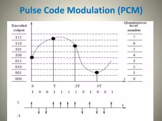
Waveform Coding • Our focus will be on Pulse-Code Modulation (PCM) • Uniform PCM • Input range for x(t): • Length of each quantization region: • is chosen as the midpoint of each quantization level • Quantization error is a random variable in the interval
Uniform PCM • Typically, N is very high and the variations of input low so that the error can be approximated as uniformly distributed on the interval • This give the quantization noise as • Signal-to-quantization noise ration (SQNR)
Uniform PCM • Example: What is the resulting SQNR for a signal uniformly distributed on [-1,1] when uniform PCM with 256 levels is employed? What is the minimum bandwidth required?
How to Improve Results • A more effective method would be to make use a non-uniform PCM: • Speech coding in the U.S. uses the µ-law compander with a typical value of µ = 255: