Download
1 / 20
210 likes | 729 Views
The General Linear Model – ANOVA for fMRI. t-tests and correlations. t-tests and correlations test basic hypotheses What about comparing more than one condition (plus a baseline)? What about testing across subjects, runs, sessions?. Design Matrix. Solution: General Linear Model. 1 ×.

E N D
t-tests and correlations t-tests and correlations test basic hypotheses What about comparing more than one condition (plus a baseline)? What about testing across subjects, runs, sessions? Design Matrix Solution: General Linear Model
1 × sequential tapping alternating tapping 2 × = General Linear Model (GLM): Logic Parcel out variance in the voxel’s time course to the contributions of two predictors plus residual noise (what the predictors can’t account for). + + + + fMRI signal residuals Design Matrix Adapted from Brain Voyager course slides
General Linear Model (GLM): Logic Models the data as a linear combination of model functions (predictors) and random noise Model functions have a known shape (our generic HRF) but amplitudes are unknown GLM is a least-squares best fit analysis of the data that best estimates the amplitudes of the predictors Aim is to minimize the sum of squares of the residuals once the model is removed (or in other words, maximise the amount of variance explained by the predictors)
blue: original time course = green: best fitting model + red: residuals General Linear Model (GLM): Logic Estimate the amplitude and variance of the predictors Remove the mean response of each predictor With amplitude estimate removed, variance of noise can be calculated – the model that minimises this measure is said to best fit the data
General Linear Model (GLM): Logic Buxton Ch. 18
GLM Baseline Here are our 2 GLM predictors shown together: Why is there no “baseline” predictor? Because if there was, the model would be overdetermined (everything would be high at some point).
GLM Baseline To understand why overdetermination is a problem, consider an example with only two states (e.g., an MT localizer comparing moving rings to stationary rings) and shifted rather than convolved with the HRF: main state predictor baseline predictor both predictors The baseline predictor is exactly the inverse of the main state predictor (the negative tail in a t-test or correlation). If we know the strength of the main state predictor, we must know the strength of the baseline predictor (baseline = main*-1) so the second predictor adds no information to our model. The problem extends to more predictors and HRF-convolved models. In the GLM, the number of predictors <= number of states - 1
GLM Output Initially, the output shows us where our model (or any part within it) accounts for a significant amount of variance:
Single Predictors We can look at voxels where a single predictor (e.g., simple tapping) accounts for a significant amount of variance:
GLM Stats For any given region, we can evaluate the GLM stats blue: original time course = green: best fitting model + red: residuals total length of sequence = 4 runs * 155 volumes = 620 volumes
GLM Stats beta = weight of predictor in model SE = standard error (variability in estimates) t = beta/SE (e.g., 1.793/.132 = 13.58) p = probability value for that level of t Entire model is significant for this region and accounts for 0.5792 = 33.5% of its variance F = t2
Combination Predictors We can look at voxels where a combination of predictors (e.g., activation to both simple AND complex finger tapping) accounts for a significant amount of variance:
GLM Combo Stats For any given region, we can evaluate the GLM stats for the combination of predictors: The sum of the 3 face predictors (1.714 + 1.103 + 1.978 = 4.795) are used in the computation of t (Note: the SE is not computed from the sum of the 3 SEs).
Contrasting Predictors We can look at voxels where a contrast between predictors (e.g., activation all face conditions vs. all place conditions) accounts for a significant amount of variance:
GLM Contrast Stats For any given region, we can evaluate the GLM stats for the contrast between predictors (like a post hoc test): Sum of the 3 face predictors minus the sum of the 3 place predictors (1.677 + 0.929 + 1.736 - 0.256 - 0.243 - 0.342 = 0.841 = 3.501) is used in the computation of t (Note: the SE is not computed from the sum of the 6 SEs).
Event-related Averaging For an area we can extract it’s time course from all trials (2 epochs/condition/run * 4 runs = 8 epochs/condition) Event-related averaging is especially valuable for event-related single trial designs. If you don’t have the same baseline before each condition, think carefully about which type to use (epoch-based may be big mistake). stimulus epoch file based epoch based -range specified in orange gives baseline with SEM bars
Flexibility of GLM • With our example data, we could ask many more questions such as: • simple vs. complex tapping • left hand vs. right hand • factorial design: • task (simple/complex) • hand (left/right) • interaction between task and hand
Multisubject Analyses • If we had additional subjects, we could compute a mutlisubject GLM • one predictor/condition • one predictor/condition/subject • one predictor/condition/run • Analysis across multiple subjects requires averaging brains in a common space: • -most common: Talairach coordinate system • You can also compare data between populations (e.g., schizophrenics vs. normals, young vs. elderly).
Advantages of General Linear Model (GLM) • can perform data analysis within and between subjects without needing to average the data itself • allows you to counterbalance orders • allows you to exclude segments of runs with artifacts • can perform more sophisticated analyses (e.g., 2 factor ANOVA with interactions) • easier to work with (do one GLM vs. many t-tests and correlations)