Download
1 / 14
140 likes | 314 Views
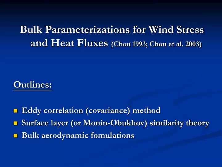
Bulk Parameterizations for Wind Stress and Heat Fluxes (Chou 1993; Chou et al. 2003) Outlines: Eddy correlation (covariance) method Surface layer (or Monin-Obukhov) similarity theory Bulk aerodynamic fomulations. Definition of parameters for bulk flux model :

E N D
Bulk Parameterizations for Wind Stress and Heat Fluxes (Chou 1993; Chou et al. 2003) Outlines: • Eddy correlation (covariance) method • Surface layer (or Monin-Obukhov) similarity theory • Bulk aerodynamic fomulations
Definition of parameters for bulk flux model: • Z -- Reference height for wind, temperature, and humidity (can be different for different variables) • U -- Surface wind speed at Z • qs -- Sea surface temperature (SST) • Qs – Sea surface saturation specific humidity (salinity, cool skin effect) • Q -- Surface air specific humidity at Z • q -- Surface air potential temperature at Z • r -- Air density • Cp -- Isobaric specific heat • Lv -- Latent heat of vaporation • CD, CH, CE– Bulk transfer coefficients for momentum, sensible and latent heat fluxes • L -- Monin-Obukhov length { = qvu*2/(gkqv*) } • k-- von Karmen constant ( =0.4) • u --kinematic viscosity of air
Eddy Correlation (Covariance) Method Wind stress t = -r <w’u’> (1a) Sensible heat flux FSH = r CP <w’T’> (1b) Latent heat flux FLH = r LV <w’q’> (1c) Where Vertical wind: w = <w> + w’ Wind speed : u = <u> + u’ Temperature: T = <T> + T’ Humidity: q = <q> + q’
Surface Layer (Monin –Obukhov) Similarity Theory Profile Scaling Parameters: Wind: u*= ( t / r )1/2 ---- t =ru*2 (2a) Temp. : q* = – FSH /(r CP u*) ---- FSH=–r Cp u* q* (2b) humidity: q*=– FLH/(r Lv u*) ----- FLH=–r Lv u*q* (2c) M-O length:L = qVu*2/(g k qV*) ---- L~ u(∂u/∂z)/<w’qV’> Z/L = 0, <w’qV’> = 0, neutral atm sfc layer (mechanical turbulence dominant) Z/L < 0, <w’qV’> < 0, unstable atm sfc layer (convective turbulence dominant) Z/L > 0, <w’qV’> > 0, stable atm sfc layer (mechanical turbulence suppressed)
Nondimensional Gradients of Wind, Potential Temperature, and Humidiy: (k Z/u*)(∂u/∂Z) = fu(Z/L) (3a) (k Z/ q*)(∂ q/∂Z) = fT(Z/L) (3b) (k Z/q*)(∂q/∂Z) = fq(Z/L) (3c) Z/L = 0, neutral, fu= fT= fq = 1 Z/L < 0, unstable, f u= (1 – 16 Z/L)-1/4 , fT= fq= (1 – 16 Z/L )-1/2 Z/L > 0,stable, fu= fT= fq = 1 + 7 Z/L von Karman constant: k = 0.40
Vertical Profiles of Wind, Potential Temperature, Humidity (U – Us)/u* = [ln(Z/Zo) –yu(Z/L)]/k (4a) (q–qs)/q* = [ln(Z/ZoT) –yT(Z/L)]/k (4b) (Q – Qs)/q* = [ln(Z/Zoq) –yq(Z/L)]/k (4c) y =∫(1 – f) d ln(Z/L), L = qv u*2/(g k qv*) * Eq.(4) obtained by adding 1 and subtracting 1 on right hand side of Eq.(3), dividing Z on Eq.(3), then integrating Eq.(3) from lower boundary (Zo, ZoT, and Zoq) to height Z.
Stability Functions:y =∫(1 – f) d ln(Z/L) Z/L = 0, neutral, yu= yT= yq= 0 Z/L > 0, stable, yu= yT= yq= -7 Z/L Z/L < 0, unstable, yu= 2 ln [ (1 + x)/2] + ln[ (1 + x2)/2] – 2 tan-1x +p/2 yT= yq= 2 ln[(1 +y)/2] x = fu-1 y = f T-1 = fq-1
Bulk Aerodynamic Formulations: Wind stresst = r CD (U–Us)2 (5a) Sensible heat flux FSH = r CP CH (U–Us) (qs–q) (5b) Latent heat flux FLH = r LV CE (U–Us) (Qs–Q) (5c) *Input parameters: U(Z), qs, q(Z), Qs, Q(Z), and Z * CD = k2/[ln(Z/ZO) –yu(Z/L)]2 (6a) CH = CD1/2 k/[ln(Z/ZOT) –yT(Z/L)] (6b) CE = CD1/2 k/[ln(Z/ZOq) –yq(Z/L)] (6c) * Eq. (6) obtained by combining Eqs. (2), (4), & (5). Us = 0.55 u* (~0)
ASTEX: Atlantic Stratocumulus Transition Experiment • COARE: Coupled Ocean-Atmosphere Response Experiment • FASTEX: Fronts and Atlantic Storm Track Experiment • JASMINE: Joint Air-Sea Monsoon Interaction Experiment • KWAJEX: Kwajalein Experiment • NAURU99: Nauru ’99 Experiment • SCOPE: San Clemente Ocean Probing Experiment • TIWE: Tropical Instability Wave Experiment • PACSF99: Pan-American Climate Study in eastern Pacific during 1999 • MOORINGS: Buoy service in the North Pacific
1913-hourly fluxes calculated from ship data using GSSTF2 bulk flux model vs observed (a) wind stresses determined by ID method, (b) latent and (c) sensible heat fluxes determined by covariance method of 10 field experiments. C: COARE F: FASTEX X: other experiments
Conclusions: • GSSTF2 bulk flux model for turbulent fluxes validated well by comparing hourly turbulent fluxes computed from research ship data with those of 10 field experiments conducted by the NOAA/ETL scientists over tropical and northern midlatitude oceans during 1991-1999 (Chou et al. 2003) • GSSTF2 bulk flux model for latent heat flux validated well by comparing hourly latent heat fluxes computed from research ship data with those of 12 field experiments conducted by NOAA/ETL and French scientists over tropical and northern midlatitude oceans during 1991-1999 (Curry et al. 2004)