Download
1 / 72
730 likes | 798 Views
Combinatorial Dominance Analysis The Knapsack Problem. Presented by: Yochai Twitto. Keywords: Combinatorial Dominance (CD) Domination number/ratio ( domn , domr ) Knapsack (KP) Incremental Insertion (II) Local Exchange (LE) PTAS Optimal Head - Greedy Tail (GRT). Overview.

E N D
Combinatorial Dominance AnalysisThe Knapsack Problem Presented by: Yochai Twitto Keywords: Combinatorial Dominance (CD) Domination number/ratio (domn, domr) Knapsack (KP) Incremental Insertion (II) Local Exchange (LE) PTAS Optimal Head - Greedy Tail (GRT)
Overview • Background • On approximations and approximation ratio. • Combinatorial Dominance • What is it ? • Definitions & Notations. • The Knapsack Problem • simple Algorithms & Analysis • Incremental Insertion • Local Exchange • PTASing • “Optimal head - greedy tail” algorithm • Summary
Overview • Background • On approximations and approximation ratio. • Combinatorial Dominance • What is it ? • Definitions & Notations. • The Knapsack Problem • simple Algorithms & Analysis • Incremental Insertion • Local Exchange • PTASing • “Optimal head - greedy tail” algorithm • Summary
Background • NP complexity class. • AA and quality of approximations. • The classical approximation ratio analysis.
NP • If P ≠ NP, then finding the optimum of NP-hard problem is difficult. If P = NP, P would encompass the NP and NP-Complete areas.
OPT Near optimal Infeasible Solutions quality line Approximations • So we are satisfied with an approximate solution. • Question: • How can we measure the solution quality ?
Solution Quality • Most of the time, naturally derived from the problem definition. • If not, it should be given as external information.
OPT Near optimal ½ OPT Infeasible Solutions quality line The classical Approximation Ratio (For maximization problem) • Assume 0 ≤ β ≤ 1. • A.r. ≥ β if • the solution quality is greater than β·OPT
Overview • Background • On approximations and approximation ratio. • Combinatorial Dominance • What is it ? • Definitions & Notations. • The Knapsack Problem • simple Algorithms & Analysis • Incremental Insertion • Local Exchange • PTASing • “Optimal head - greedy tail” algorithm • Summary
Combinatorial Dominance • What is a “combinatorial dominance guarantee” ? • Why do we need such guarantees ? • Definitions and notations.
What is a“combinatorial dominance guarantee”? • A letter of reference: • “She is half as good as I am, but I am the best in the world…” • “she finished first in my class of 75 students…” • The former is akin to an approximation ratio. • The latter to combinatorial dominance guarantee.
OPT Near optimal top O(n) Infeasible Solutions quality line What is a“combinatorial dominance guarantee”? (cont.) • We can ask: Is the returned solution guaranteed to be always in the top O(n) best solutions ?
Why do we need that ? • Assume an problem for which all solutions are at least a half as good as optimal solution. • Then, 2-factor approximating the problem is meaningless.
Corollary • The approximation ratio analysis gives us only a partial insight of the performance of the algorithm. • Dominance analysis makes the picture fuller.
Definitions & Notations • Domination number: domn • Domination ratio: domr
Domination Number: domn • Let Pbe a CO problem. • Let A be an approximation for P . • For an instance I of P, the domination numberdomn(I, A) of A on I is the number of feasible solutions of I that are not better than the solution found by A.
domn (example) • STSP on 5 vertices. • There exist 12 tours • If A returns a tour of length 7 then domn(I, A) = 8 4, 5, 5, 6, 7, 9, 9, 11, 11, 12, 14, 14 (tours lengths)
Domination Number: domn • Let Pbe a CO problem. • Let A be an approximation for P . • For any size n of P, the domination numberdomn(P, n, A) of an approximation A for P is the minimum of domn(I, A) over all instances I of P of size n.
Domination Ratio: domr • Let Pbe a CO problem. • Let A be an approximation for P . • Denote by sol(I ) the number of all feasible solutions of I. • For any size n of P, the domination ratiodomn(P, n, A) of an approximation A for P is the minimumof domn(I, A) / sol(I ) taken over all instances I of P of size n.
Overview • Background • On approximations and approximation ratio. • Combinatorial Dominance • What is it ? • Definitions & Notations. • The Knapsack Problem • simple Algorithms & Analysis • Incremental Insertion • Local Exchange • PTASing • “Optimal head - greedy tail” algorithm • Summary
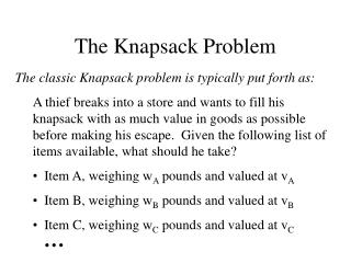
The Knapsack Problem • Instance: • Multiset of integers • Capacity • Find:
SimpleAlgorithms & Analysis • Incremental Insertion (II) • Arbitrary order • Increasing order • Decreasing order (Greedy) • Local Exchange (LE) • PTASing • “Optimal Head – Greedy Tail” (GRT)
II – Arbitrary Order • Go over the elements (arbitrary order) • Insert an element if the capacity not exceeded • Theorem:
Proof • Suppose the weights are • Let be any locally optimal solution • We may assume • Otherwise, is optimal
Proof(cont.) • Let be the largest index of a weight not belonging to Since is locally optimal
Proof(cont.) • Denote by the interval • For any solution not containing • Either • Or • That is, the number of solutions with total weight in is at most
Proof(cont.) • Solutions of weight at least are infeasible. • Solution weighted not more than are not better than
Proof(cont.) • Blackball instance: • II can lead to • Which is locally optimal blackball
Proof(cont.) • Taking the first item and omitting at least one of the rest is better. • Hence • And we finished...
II – Increasing Order • No Gain! • That was our blackball… • In the previous proof.
II - Decreasing Order (Greedy) • No drastic gain! • Blackball instance B: blackball
II - Decreasing Order (Greedy) • Greedy(B) • Weight: • Any solution taking • Exactly two elements from • Any of the last elements is better!
SimpleAlgorithms & Analysis • Incremental Insertion (II) • Arbitrary order • Increasing order • Decreasing order (Greedy) • Local Exchange (LE) • PTASing • “Optimal Head – Greedy Tail” (GRT)
Local Exchange (LE) • Assume is a solution • Allowed operations: • Insert a new element x to • Exchangex by y • x belongs to • y not belongs to • x < y
Local Exchange • Theorem:
Proof • Suppose the weights are • Let be any locally optimal solution • We may assume • Otherwise, is optimal
Proof(cont.) • Let be the largest index of a weight not belonging to Since is locally optimal
Proof(cont.) • Denote by the interval • For any solution not containing • Either • Or • That is, the number of solutions with total weight in is at most • And there are at least outside
Proof(cont.) • Let be the number of items belonging to among the first k -1 items • Let be the number of items not belonging to among the first k -1 items • How many solution pairs are of weight not belonging to ?
Proof(cont.) • We saw that • All solutions obtained by dispensing of some items from And the one obtained from them by adjoining the ’th item not belong to the interval
Proof(cont.) • So • For each of the solutions obtained from by adjoining one of the items of • Both the obtained solution • And the one obtain by adjoining it the ’th item not belong to the interval
Proof(cont.) • So • Since our solution can not be improved by local exchange • Each of the n-k solutions obtained by removing one of the last n-k items not belong to the interval • Adding each of them the ’th item we get infeasible solutions
Proof(cont.) • So
Proof(cont.) • Blackball instance: • LE can lead to • Which is locally optimal blackball
Proof(cont.) • Taking the first item and omitting at least two of the rest is better. • Hence: • And we finished... b(n)
SimpleAlgorithms & Analysis • Incremental Insertion (II) • Arbitrary order • Increasing order • Decreasing order (Greedy) • Local Exchange (LE) • PTASing • “Optimal Head – Greedy Tail” (GRT)
PTASing • There exist a PTAS for Knapsack • That is, it is possible to approximate the optimal solution to within any factor c >1 • In time polynomial in n and 1/(c -1) • We’ll see
Theorem 1 • Let be an instance of KP • Denote the weight of optimal solution by • Assume H is a factor-c approximation for KP • Then
Proof • Assume that the elements of optimal solution are labeled such that • Let ’ be the smallest integer such that