Download

1 / 31
310 likes | 526 Views
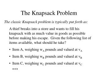
Still more dynamic programming The 0-1 knapsack problem. There are several different versions of the knapsack problem (fractional, unbounded, 0-1). We will be looking at the 0-1 problem. We are given a set of items I 1 to I n .

E N D
Still more dynamic programming The 0-1 knapsack problem
There are several different versions of the knapsack problem (fractional, unbounded, 0-1). • We will be looking at the 0-1 problem. • We are given a set of items I1 to In. • Each item Ii has a certain value vi and a certain weight wi • Our task is to select the subset of {I1 to In} that maximizes the total value of the subset while the total weight of the subset is less than or equal to the knapsack capacity C.
The foolish way to solve this problem is to test all possible subsets of {I1 to In}.However, there are 2n of them. • Is there a dynamic programming solution? • Remember, for dynamic programming to be used the problem must have optimal substructure. • At first glance, it appears this is not the case. • Consider the following example with a maximum capacity C = 20:
The optimum set of items from {I1 to I3} is {I1, I2, I3}. • The optimum set of items from {I1 to I4} is {I1, I3, I4}. This does not contain within it the optimal solution to the subproblem of {I1 to I3}, instead it contains {I1, I3}. • We need a different way of defining the problem so that {I1, I3} is the optimum solution to some subproblem.
Notice that {I1, I3} is the optimum subset of {I1 to I3} if we restrict the maximum weight of the subset to 12 or less. (12 is the most the knapsack could weigh, and still have enough capacity to add I4.) • Lets add another parameter j, which will represent the maximum weight of any subset. • Define v[i][j] to be the value of the optimum subset up to Ii having weight j or less. We want to maximize v[n][C]
Does this problem as we have defined it have optimal substructure? • Yes. Consider the optimal subset weighing j pounds. If we remove item i from it, then what can we say about the subset that remains? • It must be the most valuable subset up to Ii-1 weighing at most j – wi pounds. • Usual proof by contradiction.
Define the recursive relationship: • Base cases: v[0][j] = 0 since we are not taking any items v[i][0] = 0 since the maximum weight is 0 • Otherwise: v[i][j] = v[i-1][j] if wi > j since we cannot add Ii if wi exceeds j, the maximum weight of the subset. • Else: v[i][j] = max (v[i-1][j], v[i-1][j-wi] + vi) • Explanation: Either the optimum subset corresponding to v[i][j] contains Ii or it does not. If not, then it is the same as v[i-1][j]. If it does contain Ii then we have to 'make room' for it by building on the sub problem v[i-1][j-wi].
Lets work through an example. (Taken from - http://www.cse.unl.edu/~goddard/Courses/CSCE310J • Unlike the LCS and edit distance problems, we will not be able to build each array element using only the info in the array. • We need to keep a table listing all item weights and values and use these when filling in the array. • To keep it simple we will use 4 items with a maximum weight of 5. Items(weight, value) are (2,3)(3,4)(4,5)(5,6). • We will show the recursive formula used in bold.
j = 0 1 2 3 4 5 i = 0 1 2 3 4 First base case v[0][j] = 0 no item
j = 0 1 2 3 4 5 i = 0 1 2 3 4 Second base case v[i][0] = 0 no weight
Items: (weight, value) 1 (2,3) 2 (3,4) 3 (4,5) 4 (5,6) j = 0 1 2 3 4 5 i = 0 1 2 3 4 v[i][j] = v[i-1][j] if wi > j Else v[i][j] = max (v[i-1][j], v[i-1][j-wi] + vi)
Items: (weight, value) 1 (2,3) 2 (3,4) 3 (4,5) 4 (5,6) j = 0 1 2 3 4 5 i = 0 1 2 3 4 v[i][j] = v[i-1][j] if wi > j Else v[i][j] = max (v[i-1][j], v[i-1][j-wi] + vi)
Items: (weight, value) 1 (2,3) 2 (3,4) 3 (4,5) 4 (5,6) j = 0 1 2 3 4 5 i = 0 1 2 3 4 v[i][j] = v[i-1][j] if wi > j Else v[i][j] = max (v[i-1][j], v[i-1][j-wi] + vi)
Items: (weight, value) 1 (2,3) 2 (3,4) 3 (4,5) 4 (5,6) j = 0 1 2 3 4 5 i = 0 1 2 3 4 v[i][j] = v[i-1][j] if wi > j Else v[i][j] = max (v[i-1][j], v[i-1][j-wi] + vi)
Items: (weight, value) 1 (2,3) 2 (3,4) 3 (4,5) 4 (5,6) j = 0 1 2 3 4 5 i = 0 1 2 3 4 v[i][j] = v[i-1][j] if wi > j Else v[i][j] = max (v[i-1][j], v[i-1][j-wi] + vi)
Items: (weight, value) 1 (2,3) 2 (3,4) 3 (4,5) 4 (5,6) j = 0 1 2 3 4 5 i = 0 1 2 3 4 v[i][j] = v[i-1][j] if wi > j Else v[i][j] = max (v[i-1][j], v[i-1][j-wi] + vi)
Items: (weight, value) 1 (2,3) 2 (3,4) 3 (4,5) 4 (5,6) j = 0 1 2 3 4 5 i = 0 1 2 3 4 v[i][j] = v[i-1][j] if wi > j Else v[i][j] = max (v[i-1][j], v[i-1][j-wi] + vi)
Items: (weight, value) 1 (2,3) 2 (3,4) 3 (4,5) 4 (5,6) j = 0 1 2 3 4 5 i = 0 1 2 3 4 v[i][j] = v[i-1][j] if wi > j Else v[i][j] = max (v[i-1][j], v[i-1][j-wi] + vi)
Items: (weight, value) 1 (2,3) 2 (3,4) 3 (4,5) 4 (5,6) j = 0 1 2 3 4 5 i = 0 1 2 3 4 v[i][j] = v[i-1][j] if wi > j Else v[i][j] = max (v[i-1][j], v[i-1][j-wi] + vi)
Items: (weight, value) 1 (2,3) 2 (3,4) 3 (4,5) 4 (5,6) j = 0 1 2 3 4 5 i = 0 1 2 3 4 v[i][j] = v[i-1][j] if wi > j Else v[i][j] = max (v[i-1][j], v[i-1][j-wi] + vi)
Items: (weight, value) 1 (2,3) 2 (3,4) 3 (4,5) 4 (5,6) j = 0 1 2 3 4 5 i = 0 1 2 3 4 v[i][j] = v[i-1][j] if wi > j Else v[i][j] = max (v[i-1][j], v[i-1][j-wi] + vi)
Items: (weight, value) 1 (2,3) 2 (3,4) 3 (4,5) 4 (5,6) j = 0 1 2 3 4 5 i = 0 1 2 3 4 v[i][j] = v[i-1][j] if wi > j Else v[i][j] = max (v[i-1][j], v[i-1][j-wi] + vi)
Items: (weight, value) 1 (2,3) 2 (3,4) 3 (4,5) 4 (5,6) j = 0 1 2 3 4 5 i = 0 1 2 3 4 v[i][j] = v[i-1][j] if wi > j Else v[i][j] = max (v[i-1][j], v[i-1][j-wi] + vi)
Items: (weight, value) 1 (2,3) 2 (3,4) 3 (4,5) 4 (5,6) j = 0 1 2 3 4 5 i = 0 1 2 3 4 v[i][j] = v[i-1][j] if wi > j Else v[i][j] = max(v[i-1][j], v[i-1][j-wi] + vi)
Items: (weight, value) 1 (2,3) 2 (3,4) 3 (4,5) 4 (5,6) j = 0 1 2 3 4 5 i = 0 1 2 3 4 v[i][j] = v[i-1][j] if wi > j Else v[i][j] = max(v[i-1][j], v[i-1][j-wi] + vi)
As with most dynamic programming problems, we now know the optimum value, but not the sequence of steps that was used to achieve this optimum. • We can trace back through the table to find the items that were added. • The key is to notice that if v[i][j] = v[i-1][j] then item i is not in the knapsack. If v[i][j] ≠ v[i-1][j] then item i is in the knapsack. In this case we set j = j – wi, and i = i-1 and continue.
Items: (weight, value) 1 (2,3) 2 (3,4) 3 (4,5) 4 (5,6) j = 0 1 2 3 4 5 i = 0 1 2 3 4 v[4][5] = v[3][5] therefore item 4 is not in the knapsack.
Items: (weight, value) 1 (2,3) 2 (3,4) 3 (4,5) 4 (5,6) j = 0 1 2 3 4 5 i = 0 1 2 3 4 v[3][5] = v[2][5] therefore item 3 is not in the knapsack.
Items: (weight, value) 1 (2,3) 2 (3,4) 3 (4,5) 4 (5,6) j = 0 1 2 3 4 5 i = 0 1 2 3 4 v[2][5] ≠ v[1][5] therefore item 2 is in the knapsack. i = i-1 = 2 - 1 = 1 j = j - wi = 5 - 3 = 2
Items: (weight, value) 1 (2,3) 2 (3,4) 3 (4,5) 4 (5,6) j = 0 1 2 3 4 5 i = 0 1 2 3 4 v[1][2] ≠ v[0][2] therefore item 1 is in the knapsack. i = i - 1 = 1 - 1 = 0 j = j - wi = 2 - 2 = 0 Finished
Since the array is nxC the order of the algorithm is clearly θ(nC) where the number of items is n and the capacity of the knapsack is C. • Does anyone see anything strange about the fact that we seem to have a polynomial time algorithm for this problem? • The 0-1 knapsack problem is a known NP complete problem. How can we have a polynomial time solution? • This is a pseudo polynomial time algorithm. It depends on C as well as n, and C is unbounded. It could be 2n or n! or nn. • Nonetheless, this does give us a choice when evaluating this problem. If n is large and C is small, then the best choice is to use dynamic programming. If n is small and C large, then use some other technique.