Download
1 / 34
340 likes | 418 Views
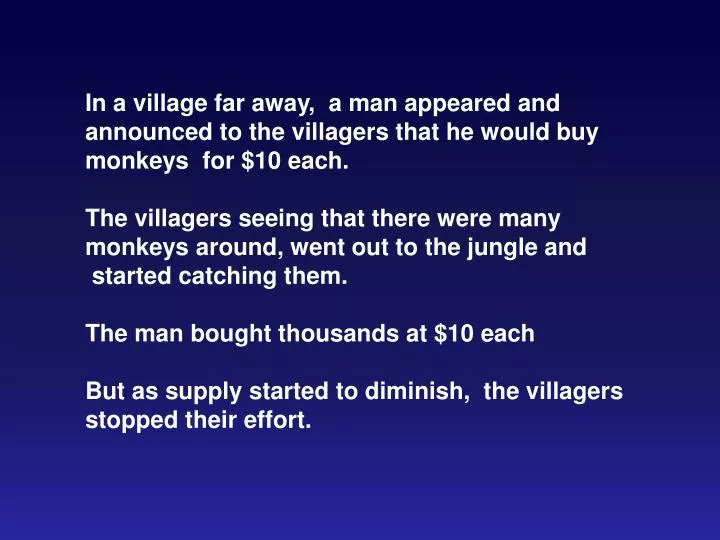
In a village far away, a man appeared and announced to the villagers that he would buy monkeys for $10 each. The villagers seeing that there were many monkeys around, went out to the jungle and started catching them. The man bought thousands at $10 each

E N D
In a village far away, a man appeared and announced to the villagers that he would buy monkeys for $10 each.The villagers seeing that there were many monkeys around, went out to the jungle and started catching them.The man bought thousands at $10 each But as supply started to diminish, the villagers stopped their effort.
The man then announced that he would pay $20 for a monkey.This renewed the efforts of the villagers and they started catching monkeys again.The supply of monkey's diminished even further and the villagers once again, stopped their effort.
The offer was then increased to $25 per monkey.The supply of monkeys became so depleted that it was an effort to even see a monkey let alone catch one!The man now announced that he would buy monkeys at $50!However, since he had to go to the city on business, and left his assistant to buy on his behalf.
The assistant told the villagers 'Look at all these monkeys that the man has collected. I will sell them to you for $35 and when the man returns from the city, you can sell them to him for $50 each.'The villagers rounded up all their savings andbought back all the monkeys.
They never saw the man nor his assistant again!Now you have a better understanding of how the stock market works..
Chapter Twelve Chapter 12
Define the Population Determine the Sampling Frame Select Sampling Technique(s) Determine the Sample Size Execute the Sampling Process Figure 12.3 Sampling Design Process
Figure 12.7 Non-probability Sampling Techniques Figure 12.7 Nonprobability Sampling Techniques Nonprobability Sampling Techniques Convenience Sampling Judgmental Sampling Quota Sampling Snowball Sampling Figure 12.9 Probability Sampling Techniques Probability Sampling Techniques Simple Random Sampling Systematic Sampling Stratified Sampling Cluster Sampling
Definitions and Symbols • Parameter: • Statistic: • Finite Population Correction: • Precision level: • Confidence interval: • Confidence level:
The Confidence Interval Approach The confidence interval is given by We can now set a 95% confidence interval around the sample mean of $182. The 95% confidence interval is given by + 1.96 = 182.00 + 1.96(3.18) = 182.00 + 6.23 Thus the 95% confidence interval ranges from $175.77 to $188.23.
0.475 0.475 _ _ _ XL X XU Figure 13.4 95% Confidence Interval
Area is 0.3413 Area between µ and µ + 1 s = 0.3431 Area between µ and µ + 2 s = 0.4772 Area between µ and µ + 3 s = 0.4986 X Scale Figure 13A.1Finding Probabilities Corresponding to Known Values
Area is 0.475 Area is 0.475 Area is 0.025 Area is 0.025 X Scale X 50 Z Scale +Z -Z 0 Figure 13A.3Finding Values Corresponding to Known Probabilities: Confidence Interval
Chapter Sixteen Chapter 16
FrequencyDistribution • In a frequency distribution, one variable is considered at a time. • A frequency distribution for a variable produces a table of frequency counts, percentages, and cumulative percentages for all the values associated with that variable.
Statistics Associated with Frequency DistributionMeasures of Location • The mean, • The mode • Median • Range • Variance • standard deviation • Type I Error • Type II Error • Power of a Test
A General Procedure for Hypothesis TestingStep 1: Formulate the Hypothesis • A null hypothesis is a statement of the status quo, one of no difference or no effect. If the null hypothesis is not rejected, no changes will be made. • An alternative hypothesis is one in which some difference or effect is expected. Accepting the alternative hypothesis will lead to changes in opinions or actions. • The null hypothesis refers to a specified value of the population parameter (e.g., ), not a sample statistic (e.g., ).
Cross-Tabulation • While a frequency distribution describes one variable at a time, a cross-tabulation describes two or more variables simultaneously. • Cross-tabulation results in tables that reflect the joint distribution of two or more variables with a limited number of categories or distinct values, e.g., Table 16.3. • chi-square • contingency coefficient • Cramer's V
Chapter Seventeen Chapter 17
t-test (var?) z-test (var) 2 group t-test F test equality of variance Paired t-test z-test z-test Chi-square Chi-square Chi-square Hypothesis Tests Related to Differences Tests of Differences One Sample Two Independent Samples Paired Samples More Than Two Samples Means Means Means Means One-way ANOVA Proportions Proportions Proportions Proportions
Statistics Associated with One-way Analysis of Variance • eta2 (2).The strength of the effects of X (independent variable or factor) on Y (dependent variable) is measured by eta2 (2).The value of 2 varies between 0 and 1. • F statistic. The null hypothesis that the category means are equal in the population is tested by an F statistic based on the ratio of mean square related to X and mean square related to error. • Mean square. This is the sum of squares divided by the appropriate degrees of freedom.
Hypothesis Testing Related to Differences • Parametric tests assume that the variables of interest are measured on at least an interval scale. • These tests can be further classified based on whether one or two or more samples are involved. • The samples are independent if they are drawn randomly from different populations. For the purpose of analysis, data pertaining to different groups of respondents, e.g., males and females, are generally treated as independent samples. • The samples are paired when the data for the two samples relate to the same group of respondents.
Chapter Eighteen Chapter 18
Product Moment Correlation • The product moment correlation,r, summarizes the strength of association between two metric (interval or ratio scaled) variables, say X and Y. • It is an index used to determine whether a linear or straight-line relationship exists between X and Y. • As it was originally proposed by Karl Pearson, it is also known as the Pearson correlation coefficient. It is also referred to as simple correlation, bivariate correlation, or merely the correlation coefficient.
Product Moment Correlation • r varies between -1.0 and +1.0. • The correlation coefficient between two variables will be the same regardless of their underlying units of measurement.
Conducting One-way Analysis of VarianceDecompose the Total Variation The total variation in Y, denoted by SSy, can be decomposed into two components: SSy = SSbetween + SSwithin where the subscripts between and within refer to the categories of X. SSbetween is the variation in Y related to the variation in the means of the categories of X. For this reason, SSbetweenis also denoted as SSx. SSwithin is the variation in Y related to the variation within each category of X. SSwithin is not accounted for by X. Therefore it is referred to as SSerror.
Figure 18.4 A Nonlinear Relationship for Which r = 0 . . 6 . . 5 4 . . 3 2 . 1 0 -3 -2 -1 0 1 2 3
Regression Analysis Regressionanalysis is used in the following ways: • Determine whether the independent variables explain a significant variation in the dependent variable: whether a relationship exists. • Determine how much of the variation in the dependent variable can be explained by the independent variables: strength of the relationship. • Determine the structure or form of the relationship: the mathematical equation relating the independent and dependent variables. • Predict the values of the dependent variable. • Control for other independent variables when evaluating the contributions of a specific variable or set of variables. • Regression analysis is concerned with the nature and degree of association between variables and does not imply or assume any causality.
Plot the Scatter Diagram Formulate the General Model Estimate the Parameters Estimate Standardized Regression Coefficients Test for Significance Determine the Strength and Significance of Association Check Prediction Accuracy Examine the Residuals Refine the Model Conducting Bivariate Regression Analysis Fig. 18.5
Plot of Attitude with Duration 9 Attitude 6 3 2.25 4.5 9 6.75 11.25 13.5 15.75 18 Duration of Car Ownership Figure 18.3
Figure 18.6 Bivariate Regression Figure 18.6 Bivariate Regression Y b0 + b1 X