Download

1 / 38
380 likes | 582 Views
Testing CAPM. Plan. Up to now: analysis of return predictability Main conclusion: need a better risk model explaining cross-sectional differences in returns Today: is CAPM beta a sufficient description of risks? Time-series tests Cross-sectional tests Anomalies and their interpretation.

E N D
Plan • Up to now: analysis of return predictability • Main conclusion: need a better risk model explaining cross-sectional differences in returns • Today: is CAPM beta a sufficient description of risks? • Time-series tests • Cross-sectional tests • Anomalies and their interpretation EFM 2006/7
CAPM • Sharpe-Lintner CAPM: Et-1[Ri,t] = RF + βi (Et-1[RM,t] – RF) • Black (zero-beta) CAPM: Et-1[Ri,t] = Et-1[RZ,t] + βi (Et-1[RM,t] – Et-1[RZ,t]) • Single-period model for expected returns, implying that • The intercept is zero • Beta fully captures cross-sectional variation in expected returns • Testing CAPM = checking that market portfolio is on the mean-variance frontier • ‘Mean-variance efficiency’ tests EFM 2006/7
Testing CAPM • Standard assumptions for testing CAPM • Rational expectations for Ri,t, RM,t, RZ,t: • Ex ante → ex post • E.g., Ri,t = Et-1Ri,t + ei,t, where e is white noise • Constant beta • Testable equations: Ri,t-RF = βi(RM,t-RF) + εi,t, Ri,t = (1-βi)RZ,t + βiRM,t + εi,t, • where Et-1(εi,t)=0, Et-1(RM,tεi,t)=0, Et-1(RZ,tεi,t)=0, Et-1(εi,t, εi,t+j)=0 (j≠0) EFM 2006/7
Time-series tests • Sharpe-Lintner CAPM: Ri,t-RF = αi + βi(RM,t-RF) + εi,t (+ δiXi,t-1) • H0: αi=0 for any i=1,…,N (δi=0) • Strong assumptions: Ri,t ~ IID Normal • Estimate by ML, same as OLS • Finite-sample F-test, which can be rewritten in terms of Sharpe ratios • Alternatively: Wald test or LR test • Weaker assumptions: allow non-normality, heteroscedasticity, auto-correlation of returns • Test by GMM EFM 2006/7
Time-series tests(cont.) • Black (zero-beta) CAPM: Ri,t = αi + βiRM,t + εi,t, • H0: there exists γ s.t. αi=(1-βi)γ for any i=1,…,N • Strong assumptions: Ri,t ~ IID Normal • LR test with finite-sample adjustment • Performance of tests: • The size is correct after the finite-sample adjustment • The power is fine for small N relative to T EFM 2006/7
Results • Early tests: did not reject CAPM • Gibbons, Ross, and Shanken (1989) • Data: US, 1926-1982, monthly returns of 11 industry portfolios, VW-CRSP market index • For each individual portfolio, standard CAPM is not rejected • Joint test rejects CAPM • CLM, Table 5.3 • Data: US, 1965-1994, monthly returns of 10 size portfolios, VW-CRSP market index • Joint test rejects CAPM, esp. in the earlier part of the sample period EFM 2006/7
Cross-sectional tests • Main idea: Ri,t = γ0 + γ1βi + εi,t (+γ2Xi,t) • H0: asset returns lie on the security market line • γ0 = RF, • γ1 = mean(RM-RF) > 0, • γ2 = 0 • Two-stage procedure (Fama-MacBeth, 1973): • Time-series regressionsto estimate beta • Cross-sectional regressions period-by-period EFM 2006/7
Time-series regressions Ri,t = αi + βiRM,t + εi,t • First 5y period: • Estimate betas for individual stocks, form 20 beta-sorted portfolios with equal number of stocks • Second 5y period: • Recalculate betas of the stocks, assign average stock betas to the portfolios • Third 5y period: • Each month, run cross-sectional regressions EFM 2006/7
Cross-sectional regressions Ri,t-RF = γ0 + γ1βi + γ2β2i + γ3σi + εi,t • Running this regression for each month t, one gets the time series of coefficients γ0,t, γ1,t, … • Compute mean and std of γ’s from these time series: • No need for s.e. of coefficients in the cross-sectional regressions! • Shanken’s correction for the ‘error-in-variables’ problem • Assuming normal IID returns, t-test EFM 2006/7
Why is Fama-MacBeth approach popular in finance? • Period-by-period cross-sectional regressions instead of one panel regression • The time series of coefficients => can estimate the mean value of the coefficient and its s.e. over the full period or subperiods • If coefficients are constant over time, this is equivalent to FE panel regression • Simple: • Avoids estimation of s.e. in the cross-sectional regressions • Esp. valuable in presence of cross-correlation • Flexible: • Easy to accommodate additional regressors • Easy to generalize to Black CAPM EFM 2006/7
Results • Until late 1970s: CAPM is not rejected • But: betas are unstable over time • Since late 70s: multiple anomalies, “fishing license” on CAPM • Standard Fama-MacBeth procedure for a given stock characteristic X: • Estimate betas of portfolios of stocks sorted by X • Cross-sectional regressions of the ptf excess returns on estimated betas and X • Reinganum (1981): • No relation between betas and average returns for beta-sorted portfolios in 1964-1979 in the US EFM 2006/7
Asset pricing anomalies EFM 2006/7
Interpretation of anomalies • Technical explanations • There are no real anomalies • Multiple risk factors • Anomalous variables proxy additional risk factors • Irrational investor behavior EFM 2006/7
Technical explanations: Roll’s critique • For any ex post MVE portfolio, pricing equations suffice automatically • It is impossible to test CAPM, since any market index is not complete • Response to Roll’s critique • Stambaugh (1982): similar results if add to stock index bonds and real estate: unable to reject zero-beta CAPM • Shanken (1987): if correlation between stock index and true global index exceeds 0.7-0.8, CAPM is rejected • Counter-argument: • Roll and Ross (1994): even when stock market index is not far from the frontier, CAPM can be rejected EFM 2006/7
Technical explanations: Data snooping bias • Only the successful results (out of many investigated variables) are published • Subsequent studies using variables correlated with those that were found significant before are also likely to reject CAPM • Out-of-sample evidence: • Post-publication performance in US: premiums get smaller (size, turn of the year effects) or disappear (the week-end, dividend yield effects) • Pre-1963 performance in US (Davis, Fama, and French, 2001): similar value premium, which subsumes the size effect • Other countries (Fama&French, 1998): value premium in 13 developed countries EFM 2006/7
Technical explanations (cont.) • Error-in-variables problem: • Betas are measured imprecisely • Anomalous variables are correlated with true betas • Sample selection problem • Survivor bias: the smallest stocks with low returns are excluded • Sensitivity to the data frequency: • CAPM not rejected with annual data • Mechanical relation between prices and returns (Berk, 1995) • Purely random cross-variation in the current prices (Pt) automatically implies higher returns (Rt=Pt+1/Pt) for low-price stocks and vice versa EFM 2006/7
Multiple risk factors • Some anomalies are correlated with each other: • E.g., size and January effects • Ball (1978): • The value effect indicates a fault in CAPM rather than market inefficiency, since the value characteristics are stable and easy to observe => low info costs and turnover EFM 2006/7
Multiple risk factors (cont.) • Chan and Chen (1991): • Small firms bear a higher risk of distress, since they are more sensitive to macroeconomic changes and are less likely to survive adverse economic conditions • Lewellen (2002): • The momentum effect exists for large diversified portfolios of stocks sorted by size and BE/ME => can’t be explained by behavioral biases in info processing EFM 2006/7
Irrational investor behavior • Investors overreact to bad earnings => temporary undervaluation of value firms • La Porta et al. (1987): • The size premium is the highest after bad earnings announcements EFM 2006/7
Fama and French(1992) "The cross-section of expected stock returns", a.k.a. "Beta is dead“ article • Evaluate joint roles of market beta, size, E/P, leverage, and BE/ME in explaining cross-sectional variation in US stock returns EFM 2006/7
Data • All non-financial firms in NYSE, AMEX, and (after 1972) NASDAQ in 1963-1990 • Monthly return data (CRSP) • Annual financial statement data (COMPUSTAT) • Used with a 6m gap • Market index: the CRSP value-wtd portfolio of stocks in the three exchanges • Alternatively: EW and VW portfolio of NYSE stocks, similar results (unreported) EFM 2006/7
Data (cont.) • ‘Anomaly’ variables: • Size: ln(ME) • Book-to-market: ln(BE/ME) • Leverage: ln(A/ME) or ln(A/BE) • Earnings-to-price: E/P dummy (1 if E<0) or E(+)/P • E/P is a proxy for future earnings only when E>0 EFM 2006/7
Methodology • Each year t, in June: • Determine the NYSE decile breakpoints for size (ME), divide all stocks to 10 size portfolios • Divide each size portfolio into 10 portfolios based on pre-ranking betas estimated over 60 past months • Measure post-ranking monthly returns of 100 size-beta EW portfolios for the next 12 months • Measure full-period betas of 100 size-beta portfolios • Run Fama-MacBeth (month-by-month) CS regressions of the individual stock excess returns on betas, size, etc. • Assign to each stock a post-ranking beta of its portfolio EFM 2006/7
Results • Table 1: characteristics of 100 size-beta portfolios • Panel A: enough variation in returns, small (but not high-beta) stocks earn higher returns • Panel B: enough variation in post-ranking betas, strong negative correlation (on average, -0.988) between size and beta; in each size decile, post-ranking betas capture the ordering of pre-ranking betas • Panel C: in any size decile, the average size is similar across beta-sorted portfolios EFM 2006/7
Results (cont.) • Table 2: characteristics of portfolios sorted by size or by pre-ranking beta • When sorted by size alone: strong negative relation between size and returns, strong positive relation between betas and returns • When sorted by betas alone: no clear relation between betas and returns! EFM 2006/7
Results (cont.) • Table 3: Fama-MacBeth regressions • Even when alone, beta fails to explain returns! • Size has reliable negative relation with returns • Book-to-market has even stronger (positive) relation • Market and book leverage have significant, but opposite effect on returns (+/-) • Since coefficients are close in absolute value, this is just another manifestation of book-to-market effect! • Earnings-to-price: U-shape, but the significance is killed by size and BE/ME EFM 2006/7
Authors’ conclusions • “Beta is dead”: no relation between beta and average returns in 1963-1990 • Other variables correlated with true betas? • But: beta fails even when alone • Though: shouldn’t beta be significant because of high negative correlation with size? • Noisy beta estimates? • But: post-ranking betas have low s.e. (most below 0.05) • But: close correspondence between pre- and post-ranking betas for the beta-sorted portfolios • But: same results if use 5y pre-ranking or 5y post-ranking betas EFM 2006/7
Authors’ conclusions • Robustness: • Similar results in subsamples • Similar results for NYSE stocks in 1941-1990 • Suggest a new model for average returns, with size and book-to-market equity • This combination explains well CS variation in returns and absorbs other anomalies EFM 2006/7
Discussion • Hard to separate size effects from CAPM • Size and beta are highly correlated • Since size is measured precisely, and beta is estimated with large measurement error, size may well subsume the role of beta! • Once more, Roll and Ross (1994): • Even portfolios deviating only slightly (within the sampling error) from mean-variance efficiency may produce a flat relation between expected returns and beta EFM 2006/7
Further research • Conditional CAPM • The ‘anomaly’ variables may proxy for time-varying market risk exposures • Consumption-based CAPM • The ‘anomaly’ variables may proxy for consumption betas • Multifactor models • The ‘anomaly’ variables may proxy for time-varying risk exposures to multiple factors EFM 2006/7
Ferson and Harvey(1998) "Fundamental determinants of national equity market returns: A perspective on conditional asset pricing" • Conditional tests of CAPM on the country level • Monthly returns on MSCI stock indices of 21 developed countries, 1970-1993 EFM 2006/7
Time series approach ri,t+1=(α0i+α’1iZt+α’2iAi,t) + (β0i+β’1iZt+β’2iAi,t) rM,t+1+εi,t+1 • Zt are global instruments • World market return, dividend yield, FX, interest rates • Ai,t are local (country-specific) instruments • E/P, D/P, 60m volatility, 6m momentum, GDP per capita, inflation, interest rates • H0: αi = 0 EFM 2006/7
Results: for mostcountries • Betas are time-varying, mostly due to local variables • E/P, inflation, long-term interest rate • Alphas are time-varying, due to • E/P, P/CF, P/BV, volatility, inflation, long-term interest rate, and term spread • Economic significance: typical abnormal return (in response to 1σ change in X) around 1-2% per month EFM 2006/7
Fama-MacBeth approach • Each month: • Estimate time-series regression with 60 prior months using one local instrument ri,t+1 = (α0i + α1iAi,t) + (β0i + β1iAi,t) rM,t+1 + εi,t+1 • Estimate WLS cross-sectional regression using the fitted values of alpha and beta and the attribute: ri,t+1 = γ0,t+1+γ1,t+1ai,t+1+γ’2,t+1bi,t+1+γ3,t+1Ai,t+ei,t+1 EFM 2006/7
Results • The explanatory power of attributes as instruments for risk is much greater than for mispricing • Some attributes enter mainly as instruments for beta (e.g., E/P) or alpha (e.g., momentum) EFM 2006/7
Conclusions • Strong support for the conditional asset pricing model • Local attributes drive out global information variables in models of conditional betas • The explanatory power of attributes as instruments for risk is much greater than for mispricing • The relation of the attributes to expected returns and risks is different across countries EFM 2006/7