Review: Uniform cost search (same as Dijkstra’s shortest path algorithm)

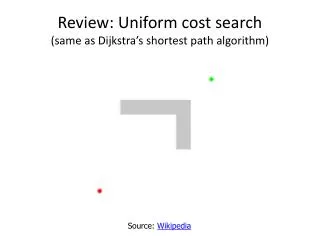
Review: Uniform cost search(same as Dijkstra’s shortest path algorithm) Source: Wikipedia

Review: Uninformed search strategies If all step costs are equal Yes O(bd) O(bd) Yes Number of nodes with g(n) ≤ C* Yes No No O(bm) O(bm) If all step costs are equal O(bd) Yes O(bd) • b: maximum branching factor of the search tree • d: depth of the optimal solution • m: maximum length of any path in the state space • C*: cost of optimal solution • g(n): cost of path from start state to node n

Informed search • Idea: give the algorithm “hints” about the desirability of different states • Use an evaluation functionto rank nodes and select the most promising one for expansion • Greedy best-first search • A* search

Heuristic function • Heuristic function h(n) estimates the cost of reaching goal from node n • Example: Start state Goal state

Heuristic for the Romania problem

Greedy best-first search • Expand the node that has the lowest value of the heuristic function h(n)

Greedy best-first search example

Properties of greedy best-first search • Complete? No – can get stuck in loops start goal

Properties of greedy best-first search • Complete? No – can get stuck in loops • Optimal? No

Properties of greedy best-first search • Complete? No – can get stuck in loops • Optimal? No • Time? Worst case: O(bm) Can be much better with a good heuristic • Space? Worst case: O(bm)

How can we fix the greedy problem?

A* search • Idea: avoid expanding paths that are already expensive • The evaluation function f(n) is the estimated total cost of the path through node n to the goal: f(n) = g(n) + h(n) g(n): cost so far to reach n (path cost) h(n): estimated cost from n to goal (heuristic)

A* search example

Another example Source: Wikipedia

Admissible heuristics • A heuristic h(n) is admissible if for every node n, h(n)≤h*(n), where h*(n) is the true cost to reach the goal state from n • An admissible heuristic never overestimates the cost to reach the goal, i.e., it is optimistic • Example: straight line distance never overestimates the actual road distance • Theorem: If h(n)is admissible, A*is optimal

Optimality of A* • Suppose A* search terminates at goal state n* with f(n*) = g(n*) = C* • For any other frontier node n, we have f(n) ≥ C* • In other words, theestimated cost f(n) of any solution path going throughnis no lower than C* • Since f(n) is an optimisticestimate, there is no way that a solution path going through ncan have an actual cost lower thanC*

Optimality of A* • A* is optimally efficient – no other tree-based algorithm that uses the same heuristic can expand fewer nodes and still be guaranteed to find the optimal solution • Any algorithm that does not expand all nodes with f(n) ≤ C* risks missing the optimal solution

Properties of A* • Complete? Yes – unless there are infinitely many nodes with f(n) ≤C* • Optimal? Yes • Time? Number of nodes for which f(n) ≤ C* (exponential) • Space? Exponential

Designing heuristic functions • Heuristics for the 8-puzzle h1(n)= number of misplaced tiles h2(n)= total Manhattan distance (number of squares from desired location of each tile) h1(start)= 8 h2(start) = 3+1+2+2+2+3+3+2 = 18 • Are h1and h2admissible?

Heuristics from relaxed problems • A problem with fewer restrictions on the actions is called a relaxed problem • The cost of an optimal solution to a relaxed problem is an admissible heuristic for the original problem • If the rules of the 8-puzzle are relaxed so that a tile can move anywhere, then h1(n)gives the shortest solution • If the rules are relaxed so that a tile can move to any adjacent square, then h2(n)gives the shortest solution

Heuristics from subproblems • Let h3(n) be the cost of getting a subset of tiles (say, 1,2,3,4) into their correct positions • Can precompute and save the exact solution cost for every possible subproblem instance – pattern database

Dominance • If h1and h2are both admissible heuristics andh2(n)≥ h1(n)for all n,(both admissible) then h2dominatesh1 • Which one is better for search? • A* search expands every node with f(n) < C* orh(n) < C* – g(n) • Therefore, A* search with h1will expand more nodes

Dominance • Typical search costs for the 8-puzzle (average number of nodes expanded for different solution depths): • d=12IDS = 3,644,035 nodes A*(h1) = 227 nodes A*(h2) = 73 nodes • d=24 IDS ≈ 54,000,000,000 nodes A*(h1) = 39,135 nodes A*(h2) = 1,641 nodes

Combining heuristics • Suppose we have a collection of admissible heuristics h1(n), h2(n), …, hm(n), but none of them dominates the others • How can we combine them? h(n) = max{h1(n), h2(n), …, hm(n)}

Weighted A* search • Idea: speed up search at the expense of optimality • Take an admissible heuristic, “inflate” it by a multiple α> 1, and then perform A* search as usual • Fewer nodes tend to get expanded, but the resulting solution may be suboptimal (its cost will be at most α times the cost of the optimal solution)

Example of weighted A* search Heuristic: 5 * Euclidean distance from goal Source: Wikipedia

Example of weighted A* search Heuristic: 5 * Euclidean distance from goal Source: Wikipedia Compare: Exact A*

Memory-bounded search • The memory usage of A* can still be exorbitant • How to make A* more memory-efficient while maintaining completeness and optimality? • Iterative deepening A* search • Recursive best-first search, SMA* • Forget some subtrees but remember the best f-value in these subtrees and regenerate them later if necessary • Problems: memory-bounded strategies can be complicated to implement, suffer from “thrashing”

All search strategies If all step costs are equal Yes O(bd) O(bd) Yes Number of nodes with g(n) ≤ C* Yes No No O(bm) O(bm) If all step costs are equal O(bd) Yes O(bd) Worst case: O(bm) No No Best case: O(bd) Yes Yes Number of nodes with g(n)+h(n) ≤ C*

Review: Uniform cost search (same as Dijkstra’s shortest path algorithm)