Download

1 / 58
620 likes | 842 Views
CS 277, Data Mining Dimension Reduction Methods. Padhraic Smyth Department of Computer Science Bren School of Information and Computer Sciences University of California, Irvine. Today’s lecture. Dimension reduction methods Motivation Variable selection methods

E N D
CS 277, Data MiningDimension Reduction Methods Padhraic Smyth Department of Computer Science Bren School of Information and Computer Sciences University of California, Irvine
Today’s lecture • Dimension reduction methods • Motivation • Variable selection methods • Linear projection techniques • Non-linear embedding methods
Dimension Reduction methods • Dimension reduction • From d-dimensional x to k-dimensional x’ , k < d • Techniques • Variable selection: • e.g., for predictive modeling: use an algorithm to find individual variables in x that are relevant to the problem and discard the rest • e.g,. Use domain knowledge to discard irrelevant variables • Linear projections • Linearly project data to a lower-dimensional space • e.g., principal components • Non-linear embedding • Use a non-linear mapping to “embed” data in a lower-dimensional space • e.g., multidimensional scaling
Dimension Reduction: why is it useful? • In general, incurs loss of information about x • so why do this? • If dimensionality p is very large (e.g., 1000’s), representing the data in a lower-dimensional space may make learning more reliable, • e.g., clustering example • 100 dimensional data • but cluster structure is only present in 2 of the dimensions, the others are just noise • if other 98 dimensions are just noise (relative to cluster structure), then clusters will be much easier to discover if we just focus on the 2d space • Dimension reduction can also provide interpretation/insight • e.g., 2d visualization purposes, e.g., very useful for scientific data analysis • Caveat: • Consider 2-step approach of (1) dimension reduction (2) followed by learning, e.g., principal components followed by classification) • In theory this may be suboptimal
Stepwise/Greedy Approaches to Variable Selection • Consider building a predictive model with k variables from d variables • We can evaluate the quality of any model by (a) fitting it to the training data, and (b) evaluating its error E (e.g., squared error) on a validation data set • Forward-variable selection • Train a model with each variable on its own and compute E each time • Select the variable that gives the lowest error E (out of the d candidates) • Now evaluate (train, compute E) adding each of the d-1 other variables to the model • Select the pair with the lowest error E out of the d-1 candidates • Continue adding variables in this manner until E starts to increase Effectively this is an “outside loop” over our training algorithm, looping over different subsets of variables…sometimes referred to as “wrapper” methods.
Stepwise/Greedy Approaches to Variable Selection • Backward-variable selection • Same procedure but in reverse • Start with all d variables in the model and at each iteration consider removing a single variable at a time. • Limitations of these stepwise/greedy approaches? • Greedy search is not necessarily optimal (the usual limitation of local search) • Computational: may require training the model O(d2) times • Could be very expensive for large d • Results may be dependent on the particular validation set being used • Alternatives • Linear projection and non-linear embedding methods (upcoming slides) • Algorithms that simultaneously do variable selection and model training, e.g., • Decision trees • Regression models with penalty functions that drive weights to 0
Basic Principles of Linear Projection x = d-dimensional (d x 1) vector of data measurements Let a = weight vector, also dimension d x 1 Assume aTa = 1 (i.e., unit norm) aTx = Sajxj = projection of x onto vector a, gives distance of projected x along a e.g., aT = [1 0] -> projection along 1st dimension aT = [0 1] -> projection along 2nd dimension aT = [0.71, 0.71] -> projection along diagonal
Example of projection from 2d to 1d x2 Direction of weight vector a x1
Projections to more than 1 dimension Multidimensional projections: e.g., if x is 4-dimensional and we want to project to 2 dimensions a1T = [ 0.71 0.71 0 0 ] a2T = [ 0 0 0.71 0.71 ] ATx -> coordinates of x in 2dim space spanned by columns of A -> linear transformation from 4dim to 2dim space where A = [a1 a2 ] with dimensions 4 x 2
Projections to more than 1 dimension Multidimensional projections: e.g., if x is 4-dimensional and we want to project to 2 dimensions a1T = [ 0.71 0.71 0 0 ] a2T = [ 0 0 0.71 0.71 ] ATx -> coordinates of x in 2dim space spanned by columns of A -> linear transformation from 4dim to 2dim space where A = [a1 a2 ] with dimensions 4 x 2 More generally, to go from d dimensions to k dimensions, we can specify k linear projections, a1,…. ak, each of length d, and A is size d x k
Principal Components Analysis (PCA) X = d times N data matrix: columns = d-dim data vectors Let a = weight vector, also dimension d Assume aTa = 1 (i.e., unit norm) aTX = projection of each column x onto vector a, = vector of distances of projected x vectors along a PCA: find vector a such that var(aTX ) is maximized i.e., find linear projection with maximal variance More generally: ATX = k times N data matrix, with x vectors projected to k-dimensional space, where size(A) = d x k PCA: find k orthogonal columns of A such that variance in the k-dimensional projected space is maximized, k < d
PCA Example Direction of 1st principal component vector (highest variance projection) x2 x1
Principal Components Analysis (PCA) Given the first principal component a1, define the 2nd principal component as the orthogonal direction a2, that has the maximal variance Continue in this fashion finding the first k components. This yields a k-dimensional projection that has the property that it is the optimal k-dimensional projection in a squared-error sense More generally: ATx= x’, a vector of size k by 1, representing the original d-dim x vector projected to a k-dimensional space, where size(A) = d by k PCA: a k-dimensional projection where we find k orthogonal columns of A such that variance in the k-dimensional projected space is maximized, k < d
PCA Example Direction of 1st principal component vector (highest variance projection) x2 x1
PCA Example Direction of 1st principal component vector (highest variance projection) x2 x1 Direction of 2nd principal component vector
How do we compute the principal components? Let C be the symmetric d x d empirical covariance matrix (from N x d data matrix) where entry(i,j) = cov(xi, xj) be the empirical covariance of (original) variables xi and xj Basic result from linear algebra: C has d eigenvectors a1,….ad each with a real-valued eigenvalue l1,…. ld > 0 Say (without loss of generality) that the eigenvalues are ordered by size, i.e.,l1 > l2 …. > ld> 0
How do we compute the principal components? Let C be the symmetric d x d empirical covariance matrix (from N x d data matrix) where entry(i,j) = cov(xi, xj) be the empirical covariance of (original) variables xi and xj Basic result from linear algebra: C has d eigenvectors a1,….ad each with a real-valued eigenvalue l1,…. ld > 0 Say (without loss of generality) that the eigenvalues are ordered by size, i.e.,l1 > l2 …. > ld> 0 Result: the ith principal components of the N x d data matrix = the ith eigenvectors ai and the amount of variance accounted for by each component i is li So: to compute the principal components, we need to compute the eigenvectors of the empirical covariance matrix
Complexity of computing Principal Components Step 1: given an N x d data matrix, compute the empirical covariance matrix C -> For each entry cov(xi, xj) , sum over N elements -> O(N) -> there are d(d+1)/2 such entries, -> O(d2) entries -> thus, O(N d2) overall to compute C Step 2: compute the eigenvalues and eigenvectors of d x d matrix C -> in general scales as O(d3), same as matrix inversion -> Overall complexity = O(N d2 + d3 ) (a) if N >> d, O(N d2) will dominate (many more data points than dimensions) (b) if d >> N, O(d3) will dominate (many more dimensions than data points)
Complexity of computing Principal Components Step 1: given an N x d data matrix, compute the empirical covariance matrix C -> For each entry cov(xi, xj) , sum over N elements -> O(N) -> there are d(d+1)/2 such entries, -> O(d2) entries -> thus, O(N d2) overall to compute C Step 2: compute the eigenvalues and eigenvectors of d x d matrix C -> in general scales as O(d3), same as matrix inversion -> Overall complexity = O(N d2 + d3 ) (a) if N >> d, O(N d2) will dominate (many more data points than dimensions) (b) if d >> N, O(d3) will dominate (many more dimensions than data points) Speed up strategies: - for sparse data matrix, we can be much faster than O(d3) - only want the first k principal components? k << d, we can use this fact
Example: Customer Movie Ratings Data d = 100,000 movies N = 10 million users Each cell is either blank (customer did not rate this movie) or has a customer rating value
20 face images • We can represent these images as an N x d matrix where • each row is an individual image • each column is a pixel value • (note: the spatial information is not being represented)
Reconstruction of First Image with 8 eigenimages Reconstructed Image Original Image
Reconstruction of another image with eigenimages Reconstructed Image Original Image
Limitations of Local Projections Any linear projection will do poorly…. … but it is clear that the data “live on” a lower-dimensional manifold
Multidimensional Scaling (MDS) • Say we have data on N objects in the form of an N x N matrix of dissimilarities • 0’s on the diagonal • Symmetric • Could either be given data in this form, or we can create such a dissimilarity matrix from our data vectors • Examples • Perceptual dissimilarity of N objects in cognitive science experiments • String-edit distance between N protein sequences
Multidimensional Scaling (MDS) • Say we have data on N objects in the form of an N x N matrix of dissimilarities • 0’s on the diagonal • Symmetric • Could either be given data in this form, or we can create such a dissimilarity matrix from our data vectors • Examples • Perceptual dissimilarity of N objects in cognitive science experiments • String-edit distance between N protein sequences • Basic Idea of MDS • Find k-dimensional coordinates for each of the N objects such that Euclidean distances in “embedded” space matches N x N matrix of dissimilarities as closely as possible • For k =2 (typical choice) we can plot our N points as a scatter plot
Multidimensional Scaling (MDS) • Objective function for MDS is “stress” S: • N points embedded in k-dimensions -> N x k locations or parameters • To find the N x k locations? • Solve optimization problem -> minimize S function • Often used for visualization, e.g., k=2, 3 Original dissimilarities Euclidean distance in new “embedded” k-dim space
Solving the MDS Optimization Problem • Optimization problem: • S is a function of N times k parameters • Find the set of N k-dimensional positions that minimize S • Notethat location and rotation are arbitrary
Solving the MDS Optimization Problem • Optimization problem: • S is a function of N times k parameters • Find the set of N k-dimensional positions that minimize S • Notethat location and rotation are arbitrary • Gradient-based Optimization • Local iterative hill-descending, e.g., move each point to decrease S, repeat • Non-trivial optimization, can have local minima, etc • Initialization: either random or heuristically (e.g., by PCA) • Complexity is O(N2 k) per iteration • Evaluate gradient in k-dimensions based on O(N2) distances • iteration = move all points locally • Fast approximate algorithms exist • eg., Landmark MDS, de Silva and Tenenbaum(2003), • works with q x N distance matrix, q << N
MDS 2-dim representation of voting records in the US House of Representatives Figure from http://en.wikipedia.org/wiki/Multidimensional_scaling
MDS for protein sequences Sequence similarity matrix (note cluster structure) MDS embedding 226 protein sequences of the Globin family (from Klock & Buhmann 1997).
MDS from human judgements of emotion similarity Figure from http://www.acrwebsite.org/
MDS of European Countries based on genetic similarity Figure from http://andrewgelman.com/2007/06/21/nations_of_euro/
Application of MDS to Music Playlists Fast embedding of sparse music similarity graphs, J. Platt, 2004 • Music database • 10k artists, 68k albums, 189k tracks • Human-assigned metadata in terms of style/subgenre/vocal-code/mood • Results in graph with 267k vertices and 3.2 million edges • Complexity of MDS, O(N2k) per iteration, is impractical here • Used fast sparse embedding (FSE) and Landmark MDS algorithms to embed data in 20 dimensions
Relation between MDS and PCA • Say our N x N matrix of dissimilarities actually represent Euclidean distances • e.g., matrix was computed based on d-dimensional distances of all pairs of rows in an N x d data matrix • This is referred to as “classic multidimensional scaling” • In this case one can show that the optimal k-dimensional MDS solution is exactly the same as the k principal components of the N x d data matrix • This suggests that MDS is doing something similar to PCA • i.e., if N x N dissimilarities are close to being Euclidean, we should expect a solution close to PCA • Other variants of MDS try to relax the Euclidean/linear nature of MDS • E.g., “non-metric” scaling where we minimize S’ where f is some monotonic function of the distances
Limitations of Local Projections Any linear projection will do poorly…. (think about what PCA will do to this data) … but it is clear that the data “live on” a lower-dimensional manifold