Dimension Reduction

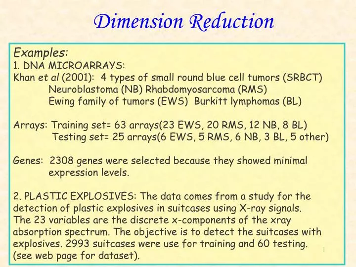
1. Dimension Reduction Examples: 1. DNA MICROARRAYS: Khan et al (2001): 4 types of small round blue cell tumors (SRBCT) Neuroblastoma (NB) Rhabdomyosarcoma (RMS) Ewing family of tumors (EWS) Burkitt lymphomas (BL) Arrays: Training set= 63 arrays(23 EWS, 20 RMS, 12 NB, 8 BL) Testing set= 25 arrays(6 EWS, 5 RMS, 6 NB, 3 BL, 5 other) Genes: 2308 genes were selected because they showed minimal expression levels. 2. PLASTIC EXPLOSIVES: The data comes from a study for the detection of plastic explosives in suitcases using X-ray signals. The 23 variables are the discrete x-components of the xray absorption spectrum. The objective is to detect the suitcases with explosives. 2993 suitcases were use for training and 60 testing. (see web page for dataset).

2. Covariance Vs Correlation Matrix • Use covariance or correlation matrix? If variables are not in the same units  Use Correlations • Dim(V) =Dim(R) = pxp and if p is large  Dimension reduction.

3. Sample Correlation Matrix Scatterplot Matrix

4. Principal Components Geometrical Intuition • - The data cloud is approximated by an ellipsoid • - The axes of the ellipsoid represent the natural components of the data • - The length of the semi-axis represent the variability of the component. Variable X2 Component1 Component2 Data Variable X1

5. DIMENSION REDUCTION • When some of the components show a very small variability they can be omitted. • The graphs shows that Component 2 has low variability so it can be removed. • The dimension is reduced from dim=2 to dim=1 Variable X2 Component1 Component2 Data Variable X1

6. Linear Algebra Linear algebra is useful to write computations in a convenient way. Singular Value Decomposition: X = U D V’ nxp nxp pxp pxp X centered =>S = V D2 V’ pxp pxp pxp pxp Principal Components(PC): Columns of V. Eigenvalues (Variance of PC’s): Diagonal elements of D2 Correlation Matrix: Subtract mean of rows of X and divide by standard deviation and calculate the covariance If p > n then SVD: X’ = U D V’ and S = U D2 U’ pxn pxn nxn nxn

7. Principal components of 100 genes. PC2 Vs PC1. (a) Cells are the observations Genes are the variables (b) Genes are the observations Cells are the variables

8. Dimension reduction: • Choosing the number of PC’s • k components explain some percentage of the variance: 70%,80%. • k eigenvalues are greater than the average (1) • Scree plot: Graph the eigenvalues and look for the last sharp decline and choose k as the number of points above the cut off. • Test the null hypothesis that the last m eigenvalues are equal (0) • The same idea can be applied to factor analysis.

9. The top 5 eigenvalues explain 81% of variability. • Five eigenvalues greater than the average 2.5% • Scree Plot • Test statistic is 4 significant for 6 and highly significant for 2. average

10. Biplots • Graphical display of X in which two sets of markers are plotted. • One set of markers a1,…,aG represents the rows of X • The other set of markers, b1,…, bp, represents the columns of X. • For example: X = UDV’X2 = U2D2V2’ • A = U2D2a and B=V2D2b, a+b=1 so X2=AB’ • The biplot is the graph of A and B together in the same graph.

11. Biplot of the first two principal components. Biplot of the first two Principal components.