Download
1 / 17
220 likes | 919 Views
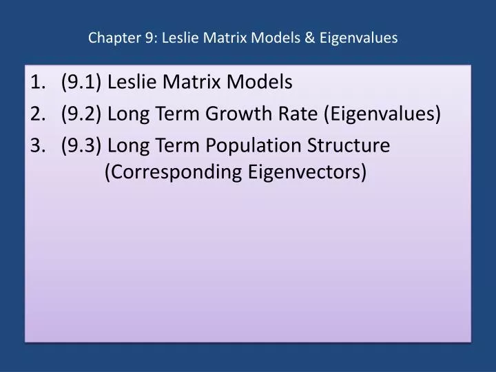
Chapter 9: Leslie Matrix Models & Eigenvalues. (9.1) Leslie Matrix Models (9.2) Long Term Growth Rate ( Eigenvalues ) (9.3) Long Term Population Structure (Corresponding Eigenvectors). 1. (9.1 ) Leslie Matrix Models. Introduction.

E N D
Chapter 9: Leslie Matrix Models & Eigenvalues • (9.1) Leslie Matrix Models • (9.2) Long Term Growth Rate (Eigenvalues) • (9.3) Long Term Population Structure (Corresponding Eigenvectors)
1. (9.1)Leslie Matrix Models Introduction • In the models presented and discussed in Chapters 6, 7, and 8, nothing is created or destroyed: • In the landscape succession examples, we never created or destroyed land; the land merely changed from one state to another • In the disease model, there were no births or deaths; individuals merely moved between infected and susceptible states • In this chapter we discuss models which take into account births and deaths
1. (9.1)Leslie Matrix Models Motivating Example: Locusts Suppose we are studying a population of locusts and want to know how their population changes over time: • Locust have three stages in their life cycle: • (1) egg • (2) nymph or hopper • (3) adult • Not all locust eggs will survive to become adults: • Some will die while they are still eggs • Others will die while they are hoppers • Locusts are only able to reproduce (lay eggs) during the adult stage of their life
1. (9.1)Leslie Matrix Models Motivating Example: Locusts Suppose in the particular population of locusts we are studying, each year: • 2% of the eggs survive to become hoppers • 5% of the hoppers survive to become adults • Adults die soon after they reproduce (i.e. they do not survive to the next year) • Additionally, the average female adult locust will produce 1000 eggs before she dies
1. (9.1)Leslie Matrix Models Motivating Example: Locusts Since it is the females that reproduce, we model only the females of the population: • Let x1(t) be the number of female eggs in the locust population at time step t • Let x2(t) be the number of female hoppers in the locust population at time step t • Let x3(t) be the number of female adults in the locust population at time step t
1. (9.1)Leslie Matrix Models Motivating Example: Locusts • We can write a system of equations to represent how this population changes each year: • As before, we express this as a matrix equation: • Now, as in the previous chapters, we are able to find how the population changes over time
1. (9.1)Leslie Matrix Models Example 9.1 (Six Years of Locusts) • How does the population of locusts change over the course of six years if there are only 50 adults at the initial time (no eggs and no hoppers)? Solution: Our initial population vector is . We want to find: We will use MATLAB to make these calculations:
1. (9.1)Leslie Matrix Models Example 9.1 (Six Years of Locusts) Here I have simply modified the file “EcoSuccessionTable”to fit our problem:
1. (9.1)Leslie Matrix Models Example 9.1 (Six Years of Locusts) Running this script, we get the output in the Command Window: Interestingly, we see that the locust population cycles every 3 years.
1. (9.1)Leslie Matrix Models Example 9.1 (Six Years of Locusts) (b) How does the population of locusts change over the course of six years if there are 50 eggs, 100 hoppers, and 50 adults at the initial time? Solution: Our initial population vector is . Simply modifying and running the script, we get the output: The population still cycles every 3 years, but the numbers are different.
1. (9.1)Leslie Matrix Models Leslie Matrices • This type of matrix population model is known as a Leslie matrix model. In general, Leslie matrices have the form: • fi is the average number of female offspring born to a female individual per time step in class i • si is the percent of individuals in class i that survive to class i+1, for i < n per time step; for i = n, sn is the proportion of individuals in class n who survive subsequent time periods • fi is the fecundity rate, and si the survival rate • Note that the first row gives the equation corresponding to the first age class x1 (like newborn)
1. (9.1)Leslie Matrix Models Example 9.2 (American Bison) • The Leslie matrix for the American Bison is given by: • The population is divided into calves, yearlings, and adults (ages two or more) • Thus, females who reach the age of 2 years survive an additional year with probability 0.95 and reproduce with the same regularity • If we start a herd with 100 adult females, what will the herd population structure look like for the subsequent five years?
1. (9.1)Leslie Matrix Models Example 9.2 (American Bison) • Solution: Our initial population vector is . • Simply modifying and running the script, we get the output: Notice that I have added a total column. The female population is growing.
2. (9.2) Long Term Growth Rate (Eigenvalues) Introduction • Given a Leslie matrix, we would like to find a stable stage distribution; that is, a distribution such that the population remains at that distribution once there • In the case of the locust population, this would mean that the fractions of the population that were eggs, hoppers and adults would stay the same through time • In Example 9.2 we saw that a Leslie matrix could model a growing population, thus we do not necessarily want to find vectors x(t) such that x(t+1) = x(t) as we did in Chapter 8 • What we want to do is find a distribution among the stage classes so that the proportion in each class does not change from one time period to the next, though the overall “number” in each class could change • If the overall population increased by a factor of λ, then each class would have increased by a factor of λ if the population were at stable stage structure
2. (9.2) Long Term Growth Rate (Eigenvalues) Introduction • A population will have this property if it satisfies the equation x(t+1) = λx(t), where the number λ is called an eigenvalue • If λ = 1, then the population is remaining constant over time (this is what occurred in the transfer matrices examples) • If λ > 1 then the population is growing over time when it is at stable stage distribution • If λ < 1, then the population is declining over time • In many contexts, λ is referred to the long-term growth rate • This notion applies only when the population is at a stable stage distribution. It may take a number of years or time steps for a population to get close to the stable stage distribution
2. (9.2) Long Term Growth Rate (Eigenvalues) Introduction • For example, suppose we have a population of children and adults and that this population has reached a stable stage distribution and currently the population vector is [25 10]T Then: (λ=1): (λ=1.5): (λ=0.5): Population size not changing; proportion children to adults: 2.5 Population size is growing; proportion children to adults: 2.5 Population size is decreasing; proportion children to adults: 2.5
2. (9.2) Long Term Growth Rate (Eigenvalues) Introduction • Let’s see if we can find these special values mathematically: This is the equation we want. I is the identity matrix. It acts like the number 1; that is, it is the multiplicative identity for matrices. See in-class notes from the document camera. It does not make sense to subtract a number from a matrix!