Download

1 / 17
170 likes | 333 Views
AP Statistics Section 3.2 C Coefficient of Determination.

E N D
A residual plot is a graphical tool for evaluating how well a linear model fits the data. The numerical quantity that tells us how well the least-squares line (LSL) does at predicting values of the response variable y is called the __________________________The symbol is ____. Some computer packages call it “_____”. coefficient of determination R-sq
We have seen instances where the least-squares regression line does not fit the data, and therefore, does not help predict the values of the response variable, y, as x changes. In such cases, our “best guess” for the value of y at any given value of x is simply ___, _____________________ the mean of the y values.
The idea of is this: How much better is the LSL at predictions then if we just used as our prediction each time?
Once again we consider the NEA vs Fat Gain example from section 3.2 A. The LSL and the lines have been drawn in the residual plot to the right. We would like to know which line comes closer to the actual y-values?
We know that the LSL minimizes the sum of the squared residuals. For this data: We will call this ____, for sum of squared errors. SSE
If we use to make predictions, then our prediction errors would be the vertical distances of the points away from the horizontal line. For this data: _________ We will call this _____, for sum of squared total variation. SST
The difference SST-SSE (in this case ________ ) shows how much the LSL reduces the total variation in the responses y.
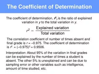
We define the coefficient of determination, r2, as the fraction of the variation in the values of y that is explained by the least-squares regression line. We can calculate r2 as follows:
We have already seen how to calculate r2 on our calculators (i.e. the same way we found r). Find r2 on your calculator for the NEA vs Fat Gain data.
A lot of factors, such as metabolism for example, affect the variation in the y-values. We can say _______ of the variation in fat gain is explained by the least-squares regression line relating fat gain and non-exercise activity. The other 39% is individual variation among the subjects that is not explained by the linear relationship.
The distinction between explanatory and response variables is essential in regression. This means we cannot reverse the roles of the two variables to make predictions. Be sure you know which variable is the explanatory.
The least-squares regression line of y on x always passes through the point ( __, __ ).
The correlation r describes the strength of a straight-line relationship. In the regression setting, the square of the correlation, r2, is the fraction of the variation in the values of y that is explained by the least-squares regression of y on x.