Download
1 / 49
490 likes | 622 Views
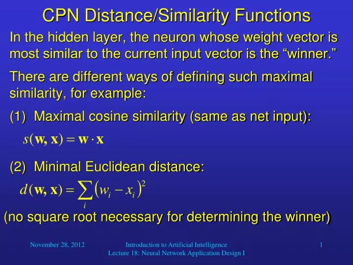
CPN Distance/Similarity Functions. In the hidden layer, the neuron whose weight vector is most similar to the current input vector is the “winner.” There are different ways of defining such maximal similarity, for example: (1) Maximal cosine similarity (same as net input):.

E N D
CPN Distance/Similarity Functions • In the hidden layer, the neuron whose weight vector is most similar to the current input vector is the “winner.” • There are different ways of defining such maximal similarity, for example: • (1) Maximal cosine similarity (same as net input): (2) Minimal Euclidean distance: (no square root necessary for determining the winner) Introduction to Artificial Intelligence Lecture 18: Neural Network Application Design I
Counterpropagation – Euclidean Distance + • Example of competitive learning with three hidden neurons: + + + 2 + 3 o o o x 1 o x x x Introduction to Artificial Intelligence Lecture 18: Neural Network Application Design I
Counterpropagation – Euclidean Distance + • Example of competitive learning with three hidden neurons: + + + 2 + 3 o o o x 1 o x x x Introduction to Artificial Intelligence Lecture 18: Neural Network Application Design I
Counterpropagation – Euclidean Distance + • Example of competitive learning with three hidden neurons: + + 2 + + 3 o o o x 1 o x x x Introduction to Artificial Intelligence Lecture 18: Neural Network Application Design I
Counterpropagation – Euclidean Distance + • Example of competitive learning with three hidden neurons: + + 2 + + 3 o o o x 1 o x x x Introduction to Artificial Intelligence Lecture 18: Neural Network Application Design I
Counterpropagation – Euclidean Distance + • Example of competitive learning with three hidden neurons: + + 2 + + 3 o o o x 1 o x x x Introduction to Artificial Intelligence Lecture 18: Neural Network Application Design I
Counterpropagation – Euclidean Distance + • Example of competitive learning with three hidden neurons: + + 2 + + 3 o o o x 1 o x x x Introduction to Artificial Intelligence Lecture 18: Neural Network Application Design I
Counterpropagation – Euclidean Distance + • Example of competitive learning with three hidden neurons: + + 2 + + 3 o o o x 1 o x x x Introduction to Artificial Intelligence Lecture 18: Neural Network Application Design I
Counterpropagation – Euclidean Distance + • Example of competitive learning with three hidden neurons: + + 2 + + 3 o o o x 1 o x x x Introduction to Artificial Intelligence Lecture 18: Neural Network Application Design I
Counterpropagation – Euclidean Distance + • Example of competitive learning with three hidden neurons: + + 2 + + 3 o o o x 1 o x x x Introduction to Artificial Intelligence Lecture 18: Neural Network Application Design I
Counterpropagation – Euclidean Distance + • Example of competitive learning with three hidden neurons: + + 2 + + 3 o o o x 1 o x x x Introduction to Artificial Intelligence Lecture 18: Neural Network Application Design I
Counterpropagation – Euclidean Distance + • Example of competitive learning with three hidden neurons: + + 2 + + 3 o o o x 1 o x x x Introduction to Artificial Intelligence Lecture 18: Neural Network Application Design I
Counterpropagation – Euclidean Distance + • Example of competitive learning with three hidden neurons: + + 2 + + 3 o o o x 1 o x x x Introduction to Artificial Intelligence Lecture 18: Neural Network Application Design I
Counterpropagation – Euclidean Distance + • Example of competitive learning with three hidden neurons: + + 2 + + 3 o o o x 1 o x x x Introduction to Artificial Intelligence Lecture 18: Neural Network Application Design I
Counterpropagation – Euclidean Distance • … and so on, • possibly with reduction of the learning rate… Introduction to Artificial Intelligence Lecture 18: Neural Network Application Design I
Counterpropagation – Euclidean Distance + • Example of competitive learning with three hidden neurons: + + 2 + + 3 o o o x 1 o x x x Introduction to Artificial Intelligence Lecture 18: Neural Network Application Design I
The Counterpropagation Network • After the first phase of the training, each hidden-layer neuron is associated with a subset of input vectors. • The training process minimized the average angle difference or Euclidean distance between the weight vectors and their associated input vectors. • In the second phase of the training, we adjust the weights in the network’s output layer in such a way that, for any winning hidden-layer unit, the network’s output is as close as possible to the desired output for the winning unit’s associated input vectors. • The idea is that when we later use the network to compute functions, the output of the winning hidden-layer unit is 1, and the output of all other hidden-layer units is 0. Introduction to Artificial Intelligence Lecture 18: Neural Network Application Design I
Counterpropagation – Euclidean Distance • At the end of the output-layer learning process, the outputs of the network are at the center of gravity of the desired outputs of the winner neuron. 2 o x o 3 o x o x x 1 + + + + + Introduction to Artificial Intelligence Lecture 18: Neural Network Application Design I
Now let us talk about… • Neural Network Application Design Introduction to Artificial Intelligence Lecture 18: Neural Network Application Design I
NN Application Design • Now that we got some insight into the theory of artificial neural networks, how can we design networks for particular applications? • Designing NNs is basically an engineering task. • As we discussed before, for example, there is no formula that would allow you to determine the optimal number of hidden units in a BPN for a given task. Introduction to Artificial Intelligence Lecture 18: Neural Network Application Design I
NN Application Design • We need to address the following issues for a successful application design: • Choosing an appropriate data representation • Performing an exemplar analysis • Training the network and evaluating its performance • We are now going to look into each of these topics. Introduction to Artificial Intelligence Lecture 18: Neural Network Application Design I
Data Representation • Most networks process information in the form of input pattern vectors. • These networks produce output pattern vectors that are interpreted by the embedding application. • All networks process one of two types of signal components: analog (continuously variable) signals or discrete (quantized) signals. • In both cases, signals have a finite amplitude; their amplitude has a minimum and a maximum value. Introduction to Artificial Intelligence Lecture 18: Neural Network Application Design I
max min max min Data Representation • analog discrete Introduction to Artificial Intelligence Lecture 18: Neural Network Application Design I
Data Representation • The main question is: • How can we appropriately capture these signals and represent them as pattern vectors that we can feed into the network? • We should aim for a data representation scheme that maximizes the ability of the network to detect (and respond to) relevant features in the input pattern. • Relevant features are those that enable the network to generate the desired output pattern. Introduction to Artificial Intelligence Lecture 18: Neural Network Application Design I
Data Representation • Similarly, we also need to define a set of desired outputs that the network can actually produce. • Often, a “natural” representation of the output data turns out to be impossible for the network to produce. • We are going to consider internalrepresentation and externalinterpretation issues as well as specific methods for creating appropriate representations. Introduction to Artificial Intelligence Lecture 18: Neural Network Application Design I
Internal Representation Issues • As we said before, in all network types, the amplitude of input signals and internal signals is limited: • analog networks: values usually between 0 and 1 • binary networks: only values 0 and 1allowed • bipolar networks: only values –1 and 1allowed • Without this limitation, patterns with large amplitudes would dominate the network’s behavior. • A disproportionately large input signal can activate a neuron even if the relevant connection weight is very small. Introduction to Artificial Intelligence Lecture 18: Neural Network Application Design I
External Interpretation Issues • From the perspective of the embedding application, we are concerned with the interpretation of input and output signals. • These signals constitute the interface between the embedding application and its NN component. • Often, these signals only become meaningful when we define an external interpretation for them. • This is analogous to biological neural systems: The same signal becomes completely different meaning when it is interpreted by different brain areas (motor cortex, visual cortex etc.). Introduction to Artificial Intelligence Lecture 18: Neural Network Application Design I
External Interpretation Issues • Without any interpretation, we can only use standard methods to define the difference (or similarity) between signals. • For example, for binary patterns x and y, we could… • … treat them as binary numbers and compute their difference as | x – y | • … treat them as vectors and use the cosine of the angle between them as a measure of similarity • … count the numbers of digits that we would have to flip in order to transform x into y (Hamming distance) Introduction to Artificial Intelligence Lecture 18: Neural Network Application Design I
External Interpretation Issues • Example: Two binary patterns x and y: • x = 00010001011111000100011001011001001y = 10000100001000010000100001000011110 • These patterns seem to be very different from each other. However, given their external interpretation… x y …x and y actually represent the same thing. Introduction to Artificial Intelligence Lecture 18: Neural Network Application Design I
Creating Data Representations • The patterns that can be represented by an ANN most easily are binary patterns. • Even analog networks “like” to receive and produce binary patterns – we can simply round values < 0.5 to 0 and values 0.5 to 1. • To create a binary input vector, we can simply list all features that are relevant to the current task. • Each component of our binary vector indicates whether one particular feature is present (1) or absent (0). Introduction to Artificial Intelligence Lecture 18: Neural Network Application Design I
Creating Data Representations • With regard to output patterns, most binary-data applications perform classification of their inputs. • The output of such a network indicates to which class of patterns the current input belongs. • Usually, each output neuron is associated with one class of patterns. • For any input, only one output neuron should be active (1) and the others inactive (0), indicating the class of the current input. Introduction to Artificial Intelligence Lecture 18: Neural Network Application Design I
Creating Data Representations • In other cases, classes are not mutually exclusive, and more than one output neuron can be active at the same time. • Another variant would be the use of binary input patterns and analog output patterns for “classification”. • In that case, again, each output neuron corresponds to one particular class, and its activation indicates the probability (between 0 and 1) that the current input belongs to that class. Introduction to Artificial Intelligence Lecture 18: Neural Network Application Design I
Creating Data Representations • Tertiary (and n-ary) patterns can cause more problems than binary patterns when we want to format them for an ANN. • For example, imagine the tic-tac-toe game. • Each square of the board is in one of three different states: • occupied by an X, • occupied by an O, • empty Introduction to Artificial Intelligence Lecture 18: Neural Network Application Design I
Creating Data Representations • Let us now assume that we want to develop a network that plays tic-tac-toe. • This network is supposed to receive the current game configuration as its input. • Its output is the position where the network wants to place its next symbol (X or O). • Obviously, it is impossible to represent the state of each square by a single binary value. Introduction to Artificial Intelligence Lecture 18: Neural Network Application Design I
Creating Data Representations • Possible solution: • Use multiple binary inputs to represent non-binary states. • Treat each feature in the pattern as an individual subpattern. • Represent each subpattern with as many positions (units) in the pattern vector as there are possible states for the feature. • Then concatenate all subpatterns into one long pattern vector. Introduction to Artificial Intelligence Lecture 18: Neural Network Application Design I
Creating Data Representations • Example: • X is represented by the subpattern 100 • O is represented by the subpattern 010 • <empty> is represented by the subpattern 001 • The squares of the game board are enumerated as follows: Introduction to Artificial Intelligence Lecture 18: Neural Network Application Design I
Creating Data Representations • Then consider the following board configuration: It would be represented by the following binary string: 100 100 001 010 010 100 001 001 010 Consequently, our network would need a layer of 27 input units. Introduction to Artificial Intelligence Lecture 18: Neural Network Application Design I
Creating Data Representations • And what would the output layer look like? • Well, applying the same principle as for the input, we would use nine units to represent the 9-ary output possibilities. • Considering the same enumeration scheme: Our output layer would have nine neurons, one for each position. To place a symbol in a particular square, the corresponding neuron, and no other neuron, would fire (1). Introduction to Artificial Intelligence Lecture 18: Neural Network Application Design I
Creating Data Representations • But… • Would it not lead to a smaller, simpler network if we used a shorter encoding of the non-binary states? • We do not need 3-digit strings such as 100, 010, and 001, to represent X, O, and the empty square, respectively. • We can achieve a unique representation with 2-digits strings such as 10, 01, and 00. Introduction to Artificial Intelligence Lecture 18: Neural Network Application Design I
Creating Data Representations • Similarly, instead of nine output units, four would suffice, using the following output patterns to indicate a square: Introduction to Artificial Intelligence Lecture 18: Neural Network Application Design I
Creating Data Representations • The problem with such representations is that the meaning of the output of one neuron depends on the output of other neurons. • This means that each neuron does not represent (detect) a certain feature, but groups of neurons do. • In general, such functions are much more difficult to learn. • Such networks usually need more hidden neurons and longer training, and their ability to generalize is weaker than for the one-neuron-per-feature-value networks. Introduction to Artificial Intelligence Lecture 18: Neural Network Application Design I
Creating Data Representations • On the other hand, sets of orthogonal vectors (such as 100, 010, 001) can be processed by the network more easily. • This becomes clear when we consider that a neuron’s input signal is computed as the inner product of the input and weight vectors. • The geometric interpretation of these vectors shows that orthogonal vectors are especially easy to discriminate for a single neuron. Introduction to Artificial Intelligence Lecture 18: Neural Network Application Design I
Creating Data Representations • Another way of representing n-ary data in a neural network is using one neuron per feature, but scaling the (analog) value to indicate the degree to which a feature is present. • Good examples: • the brightness of a pixel in an input image • the output of an edge filter • Poor examples: • the letter (1 – 26) of a word • the type (1 – 6) of a chess piece Introduction to Artificial Intelligence Lecture 18: Neural Network Application Design I
Creating Data Representations • This can be explained as follows: • The way NNs work (both biological and artificial ones) is that each neuron represents the presence/absence of a particular feature. • Activations 0 and 1 indicate absence or presence of that feature, respectively, and in analog networks, intermediate values indicate the extent to which a feature is present. • Consequently, a small change in one input value leads to only a small change in the network’s activation pattern. Introduction to Artificial Intelligence Lecture 18: Neural Network Application Design I
Creating Data Representations • Therefore, it is appropriate to represent a non-binary feature by a single analog input value only if this value is scaled, i.e., it represents the degree to which a feature is present. • This is the case for the brightness of a pixel or the output of an edge detector. • It is not the case for letters or chess pieces. • For example, assigning values to individual letters (a = 0, b = 0.04, c = 0.08, …, z = 1) implies that a and b are in some way more similar to each other than are a and z. • Obviously, in most contexts, this is not a reasonable assumption. Introduction to Artificial Intelligence Lecture 18: Neural Network Application Design I
Creating Data Representations • It is also important to notice that, in artificial (not natural!), completely connected networks the order of features that you specify for your input vectors does not influence the outcome. • For the network performance, it is not necessary to represent, for example, similar features in neighboring input units. • All units are treated equally; neighborhood of two neurons does not imply to the network that these represent similar features. • Of course once you specified a particular order, you cannot change it any more during training or testing. Introduction to Artificial Intelligence Lecture 18: Neural Network Application Design I
Creating Data Representations • If you wanted to represent the state of each square on the tic-tac-toe board by one analog value, which would be the better way to do this? • <empty> = 0 • X = 0.5 • O = 1 X = 0 <empty> = 0.5 O = 1 Not a good scale!Goes from “neutral” to“friendly” and then“hostile”. More natural scale!Goes from “friendly” to“neutral” and then“hostile”. Introduction to Artificial Intelligence Lecture 18: Neural Network Application Design I
Representing Time • So far we have only considered static data, that is, data that do not change over time. • How can we format temporal data to feed them into an ANN in order to detect spatiotemporal patterns or even predict future states of a system? • The basic idea is to treat time as another input dimension. • Instead of just feeding the current data (time t0) into our network, we expand the input vectors to contain n data vectors measured at t0,t0 - t, t0 - 2t, t0 - 3t, …, t0 – (n – 1)t. Introduction to Artificial Intelligence Lecture 18: Neural Network Application Design I
$1,000 ? t0-6t t0-5t t0-4t t0-3t t0-2t t0-t t0 t0+t Representing Time • For example, if we want to predict stock prices based on their past values (although other factors also play a role): $0 t Introduction to Artificial Intelligence Lecture 18: Neural Network Application Design I