NUMERIC AL ANAL YSIS OF PROCES SES

1. NUMERICAL ANALYSISOF PROCESSES NAP4 NONLINEAR MODELS of systems described by ordinary differential equations Initial problem (Runge Kutta, Adams) Time delay Strange attractors Rudolf Žitný, Ústav procesní a zpracovatelské techniky ČVUT FS 2010

2. Models ODE initial problem NAP4 Systems which are described by a system of ordinary differential equations and their solutions are fully described by the initial state, are for example integral models of mass and enthalpy balances elementary units ("lumped parameter" or "compartment" models). The aim is to determine the evolution of state variables (concentration, temperature) at the time, so it is an evolutionary problems. These elementary units may be specific devices (reactors, absorbers, columns, tanks, filters, ...) in "spread sheets" or zones in apparatuses in which the state can be characterized by mean temperature, and the concentration of components (ideal mixers, plug flow zone). An example is the description of a stirred vessel system of ideal mixers below and above a turbine stirrer or a replacement shell and tube heat exchanger by a systém of elementary exchangers between the baffles. Each elementary unit correspond to ordinary differential equations describing the mass balance (one for each component of the differential equation describing the rate of change of concentration) and a enthalpy balance (or total energy balance) describing temperature evolution in the department volumetric flowrate from neigbouring compartments volumetric hear source wnthalpic flows from neighbouring compartments

3. Models ODE initial problem NAP4 A system need not be described by ordinary differential equations with only first derivatives. Eg. the equations of vibration include also the second time derivative (acceleration) But every such equation can be replaced by a system of equations with only first derivatives, e.g. The initial problem is characterized by the fact that each computed variable corresponds to one differential equation of the first order and to one initial condition (value) corresponding to the initial state. …or how many equations so many initial conditions corresponding to one value of independent variable.

4. Models ODE initial problem NAP4 backmixing model (dispersion, diffusiion) Example of continuous system: (1+r+b)Q 6 5 (1+r)Q 4 2 1 Q,x(t) bQ Ci, Ti sQ rQ 3 7 model of stagnant zone recirkulation with transport delay Differential equations for concentrations Parametersdetermining distribution of flowrates (s-stagnant zone, r-recirculation, b-backmixing) must be specified, r-from flowmeter measurement, b-from correlations. Also the volume of individual compartments must be known. These parameters are most frequently identiofied from fit of predicted characteristics (for example RTD - residence time distribution) with experiment.As a result information about the size of dead zones, recirculation zones, shortcuts, intensity of dispersion etc. are obtained.

5. Models ODE Fourier transform NAP4 The models can be solved by the Fourier transformation method (see previous lecture NAZP3). It is not enough to apply only a convolution, because the model includes compartments with back mixing, stagnant zone ... However, you can come out of these differential equations, transformed by FFT. For the Fourier transform of derivation applies (assuming that the concentration at time zero is infinity) Differential equations are transformed to algebraic equations, where instead of time t is frequency f. This system of algebraic equations (linear!) is already fairly easy to solve, and the result will be the Fourier transform of concentration. Concentration courses in time are then get back by FFT. The solution is accurate and fast (using FFT), but is limited to linear models. The procedure is preferred when the coefficients of the system (r, b, s) are constant. Otherwise, it was necessary to compute the Fourier transform of the product of two functions (and it is not equal to the product of the transformation). In the general case with nonlinear terms is therefore better to stay in the time domain and seek solutions to the numerical integration of the ODE.

6. Models ODE Laplace transform NAP4 Similar relationships hold also for Laplace transform: the same convolution, correlation and transformation of derivatives Inverse Laplace transform is usually searched in dictionaries, for example

7. ODEinitial problem numerical solutions c c ck ck t t tk+1 tk+1 tk tk NAP4 One-step methods approximate solution at time tk+1=tk+ by estimating mean value of derivativein interval<tk,tk+1> Euler metodsare easily programmable even in Excel first order of accuracy means that the error is directly proportional to the step when you write a Taylor expansion for one time step, the error is O(2), a second-order accuracy. Errors, however, accumulate, so 1/ steps will result in an error O(). Euler method explicit order of accuracy (first) stableonly for small integration steps  Euler method implicit order of accuracy (first) stable, but iterations are necessary (because ck+1is unknown)

8. ODEinitial problem numericalsolutions c ck t tk+1 tk NAP4 One-step methods approximate solution at time tk+1=tk+ by estimating mean value of derivativein interval<tk,tk+1> Runge Kuttamethods calculate mean value of derivative as a weighted average of derivatives f(t,c). The most often used version calculates four points (endpoints tk, tk+1 and two midpoints at tk+1/2) This variant is implemented in MATLABu as a functionode45 Weight coefficients (1/6,1/3,1/3,1/6) andincrements c aredesigned so that the order of accuracy is the highest (4th order of accuracy in this case). Generally, the order of accuracy of RK methods is the same as the number of evaluated points.

9. ODEinitial problem numerical solutions c ck ck-1 t tk+1 tk-2 tk-1 tk NAP4 Multistep methods approximate solution at time tk+1on the basis of several previous values for example at times tk, tk-1 (two), or tk-2 (three-step method). This is usually a combination of predictor (explicit) and corrector (default formula with higher precision and stable) it is sufficient to evaluatejust one value Both formulas are second order accuracy but corrector (implicit formula) has the absolute value of the error about 9-fold lower (implicit formulas tend to have an error less than explicit, even if the order errors is the same). The disadvantage is that for the first two steps a single-step method, for example RK, must be used. On the other hand, number of computed derivatives is smaller.

10. ODEinitial problem numerical solutions NAP4 Dynamic adjustment of integration step The simplest solution is that each step is performed twice, once with step  and then with increments /2 (twice). If the difference is greater than the specified tolerance, the step  shrinks. Using the two calculated values (for full and half step) the accuracy of the final value can be improved by so called Aitken extrapolation. MATLAB uses a dynamic choice of the time step automatically. Stiff problem When you solve a system of equations may be that the integration step is dictated by the equation with an extremely short time constant, and the stability of the solution then requires extremely short integration step (the calculation time is prohibitively increased). We say that the system is stiff. Some methods of integrating ODE this unpleasant impact suppresses (an example is Gearova method). Transport delay (time shift) Time delay was included in the previous example. In this case the solver should remember the whole history of calculated results and not only the last step. Even the values for negative times (before the initial time) have to be defined.

11. ODE initial problem numerical solutions NAP4 Stability analysis Consider a differential equation describing e.g. the rate of a chemical reaction of the first order stabilitycondition restriction of time step (coef. of gain less than 1) Euler explicit integration formula of the first order Euler implicit integration formulaof the first order gain less than 1 for arbitrary 

12. ODEexamples in MATLAB NAP4 ode45, ode23Runge-Kutta (one step method with different order of accuracy) ode113Adams (multistep method) ode15sStiff (Gear multistep methodwith variable accuracy order-suitable for stiff problems) dde23transport delay

13. RTD series of mixers 1/4 x(t) y(t) (t) c1 c2 c3 c4 NAP4 An example has been solved in the previous lectures using FFT. Series 4 ideally mixed vessels (container volume, flow rate Q). The aim is to find the time courses of concentrations c1,…,c4for arbitrary initial conditions and for arbitrary course of concentration at inlet x(t). Mass balances tm=2 odpovídá poměru V/Q=0.5 (to je střední doba prodlení jedné nádoby) As an initial concentration x(t) is applied impulse response of a set of two mixers (the same volume of tanks) and zero initial concentration in all tanks. The reason for such an assignment is that there is an analytical solution that can be compared with the results of numerical solution of the ODE. Stimulus function x(t) is the impulse response of E (t) for N=2 and tm=1; outletconcentration y(t)=c4(t) shou;ld be impulse response for N=6 and tm=3

14. RTD series of mixers2/4 NAP4 MATLAB provides for the solution of ODE variety of methods (ode45, ode113, ode15s, ...) which can automatically adjust the integration step so as to achieve the required accuracy. Procedure is always the same, first define a function whose output is the vector of first derivatives for a given value of integration variable (time) and a solution vector. In our case it is necessary to define a function whose result is a column vector (4x1) of right-hand sides of 4 differential equations. It will be assumed that the stimulus function x(t) is the impulse response of nx series mixers, with a mean timetmx. The parameter tm is the mean time of the modeled system of 4 mixers. function dy = serie4(t,y,tm,tmx,nx) dy = zeros(4,1); xx=efun(t,tmx,nx); tm1=tm/4; dy(1)=(xx-y(1))/tm1; dy(2)=(y(1)-y(2))/tm1; dy(3)=(y(2)-y(3))/tm1; dy(4)=(y(3)-y(4))/tm1; It would probably be smarter if the stimulus function x(t) was directly the next formal parameter of the function serie4. I have a little problem with that in Matlab, I need advice. The Efun function can be defined as a sub-function in the m-file serie4.m, but maybe it's better to define it as a separate m-file efun.m function y=efun(t,tm,n) y=n^n*t^(n-1)/(factorial(n-1)*tm^n)*exp(-t*n/tm);

15. RTD series of mixers3/4 NAP4 Integration ODE by Runge Kutta method Sol = ode45(function describing right side, time range, initial conditions) in our case for example sol=ode45(@(t,y)serie4(t,y,2,1,1),[0 10],[0 0 0 0]) Vector of initial conditions (zero concentrations) solver: 'ode45' extdata: [1x1 struct] x: [1x29 double] y: [4x29 double] stats: [1x1 struct] idata: [1x1 struct]. Integration from t=0, to t=10. It is not possible to specify a constant integration step in Matlab Using a function as an actual parameter looks a bit strange in Matlab. It is not possibleto write simply the name of this function (serie4) because ode45 expects only two parameters (t, y) and the function serie4 has 5 parameters. Therefore, the so-called anonymous function@(t,y)expression.must be used. Result is the structuresolcontaining vector of time steps sol.x (in this specific case 29 steps was necessary for prescribed accuracy) and a corresponding matrix sol.y of calculated concentrations (four rows for four concentrations)

16. RTD series of mixers4/4 NAP4 Numerical solution by Runge Kutta (ode45) can be compared with the analytical solution E(t) for N=6 and tm=3 This is demonstration how to define a one-line function (without using a m-file) e=@(t,tm,n) n^n.*t.^(n-1)./(factorial(n-1)*tm^n).*exp(-n.*t/tm) t=linspace(0,10.23,1024); y=e(t,3,6); Standard function linspace generates vector of 1024 equidistant time steps Sy=deval(sol,t) these points are results ofode45with automatically adjusted integration time steps functiondeval interpolatesthe nonequidistant results sol.y according to the prescribed time scale t

17. RTDtime delay (transport delay) NAP4 In the case that there are time delays (long connecting pipelines, recycles) it is not possible to use the standard integration functions (ode23,ode45,…), but a different „family“ of MATLAB functions which is capable to save previous results (with prescribed vector of time delays1 2 …)

18. RTDdelay in recycle 1/2 x(t) (1+r)Q 1 2 Q rQ NAP4 Example: continuous system formed by two mixed tanks with time delay in recycle. It is quite common: connecting pipelines are usually modeled by a time delay. The aim is to find time courses of concentrations c1(t), c2(t), for given flowrate (Q), recirculation ratio (r) and volume of tanks (V1,V2), for prescribed time course of inlet concentration x(t). The system is described by the mass balances: time delay

19. RTDdelay in recycle 2/2 NAP4 Special ODE solvers must be used in MATLAB (dde23fora constant time delay, andddesdfor variabl;e time delay) sol=dde23(@derivatives, [1, 2…], history for t<tmin, [tmin,tmax]) function dcdt=dclag(t,c,z) q=1; v1=2; v2=1; r=10; if t<.2 x=1; else x=0; end dcdt=zeros(2,1); clag=z(:,1); dcdt(1)=q/v1*(x-c(1)); dcdt(2)=q/v2*(c(1)+r*clag(2)-(1+r)*c(2)); q-flowrate,v1,v2 volumes, r-recycle ratio, impulse stimulus function x(t) with duration 0.2 seconds z is the matrix of solutions in times t-k. Column index (1) is the index in vector of delays zero history c1=c2=0 for t<0 sol=dde23(@dclag,1,[0;0],[0,20]) plot(sol.x,sol.y) vector of delays1=1 (there is only one delay)

20. Trajectoryofparticles NAP4 The initial problem isalso description of motion of particles under action of forces. Examples are trajectory of droplets in the spray drying chamber, motion of particles in a fluidized bed, burning coal particles in the combustion chamber, particles in the mixer, a settling tank, etc. The equations of motion are ODE of the type: acceleration buoyant, centrifugal, electrical forces drag for in fluid moving with velocity v

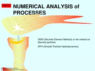
21. Trajectories of particles NAP4 In the last lecture of the course we will pay attention to the type of modern methods of DEM (Discrete Element Method), which simulates the dynamic behavior of particulate systems such as hoppers, silos, mills, mixers, separators, solid and fluid bed. Calculations are based on the solution of ordinary differential equations of motion and the consideration of interactions of individual particles. Verlet integration of dynamic equations

22. Theory of chaos strange attractor NAP4 Trajectories of particles calculated alsothe meteorologist E.Lorenz (1963) who tried to model the natural convection in atmosphere, the layer of air that is heated from below and cooled from above. After drastic simplificationshe obtained the three ordinary differential equations for the coordinates x, y, z of a particle in the atmosphere Rayleigh-Bénárdova instability The model has only 3 parameters, Rayleigh number Ra, Prandtl number Pr and the parameter b is a slenderness ratio of rotating cells. These 3 equations can be solve easily in MATLAB see next slide…

23. Theory of chaos strange attractor NAP4 trajektory pf particle fopr Ra=10, Pr=28, b=8/3 function dy = chaos(t,y) dy = zeros(3,1); dy(1) = 10*(y(2)-y(1)); dy(2) = -y(1)*y(3)+28*y(1)-y(2); dy(3) = y(1)*y(2)-8/3*y(3); sol=ode45(@chaos,[0 30],[.10001 .1 .1]) plot(sol.y(2,:),sol.y(3,:)) tt=linspace(0,30,3000); sy=deval(sol,tt); plot(sy(2,:),sy(3,:)) initial coordinates x,y,z integration up to 30 s plot graph y-z fro automatically calculated integration steps

24. Theory of chaos strange attractor NAP4 Numerically calculated trajectories behave erratically for Pr> 1 (they do not converge to a trivial steady steate solution x = y = z = 0), but they create something that looks like a counter-rotating swirls of final dimensions, and these seemingly random trajectories "jump" from the left to the right wing, and never intersect. The trajectories are extremely sensitive to initial conditions and to any disturbances (including approximation errors of numerical integration). This limiting state is called „strange attractor“ parametric trajectoryof particle z Such behavior (deterministic chaos) appears at nonlinear systemswhen a stability limit is exceeded (eg Prantl, Reynolds or Rayleigh numbers). Deterministic chaos is typical for turbulent flow. y

25. EXAM NAP 4 ODE Initial problem numerical solutions, stability

26. Exam - remember NAP4 Fourier transform of derivatives What is it initial problem What is it order of accuracy O(n) Explicit and implicit Euler method Principles of RK and multistep methods (predictor, corrector) Principle of stability analysis Principle of integration step optimisation