Download
1 / 47
470 likes | 576 Views
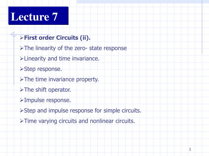
Lecture 7. First order Circuits (ii). The linearity of the zero- state response Linearity and time invariance. Step response. The time invariance property. The shift operator. Impulse response. Step and impulse response for simple circuits.

E N D
Lecture 7 • First order Circuits (ii). • The linearity of the zero- state response • Linearity and time invariance. • Step response. • The time invariance property. • The shift operator. • Impulse response. • Step and impulse response for simple circuits. • Time varying circuits and nonlinear circuits.
+ C v R=1/G is - Linearity of the Zero-state Response The zero-state response of any linear circuit is a linear function of the input; that is, the dependence of the waveform of the zero-state response on the input waveform is expressed by linear function. Any independent source in a linear circuit is considered as an input. Let illustrate this fact with the linear time-invariant RC circuit that we studied (See Fig.7.1) Let the input be the current waveform is (), and let the response be the voltage waveform v(). The zero-response state of the linear time-invariant parallel RC circuit is a linear is a linear function of the input: that is the dependence of the zero-response waveform on the input waveform has the property of additivity and homogeneity Fig.7.1 Linear time-invariant RC circuit with input isand response v
1. Let us check additivity. Consider two input currents i1 and i2 that are both applied at t0. Note that by i1 (and also i2 )we mean current waveform that starts at t0 and goes forever. Call v1 and v2 the corresponding zero-state responses. By definition, v1is the unique solution of the differential equation (7.1) with (7.2) Similarly, v2 is the unique solution of (7.3) with (7.4) Adding (7.1) and (7.3), and taking (7.2) and (7.4) into account, we see that the function v1+v2 satisfies (7.5)
with (7.6) By definition the zero-state response to the input i1+i2 applied at t=t0 is the unique solution of the differential equation (7.7) with (7.8) By the uniqueness theorem for the solution of such differential equations and by comparing (7.5) and (7.6) with (7.7) and (7.8), we arrive at the conclusion that the waveform v1()+v2() is the zero-state response to the input waveformi1()+i2(). Since this reasoning applies to any input i1() andanyi2() applied at any time t0, we have shown that the zero-state response of the RC circuit is a function of the input, which obeys the additivity property. 2. Let us check homogeneity. We consider the input i1() (applied at t0) and the input ki1() , where k is an arbitrary real constant.
By definition, the zero-state response due to i1 satisfies (7.1) and (7.2). Similarly, the zero-state response due to ki1() satisfies the differential equation (7.9) with (7.10) By multiplying (7.1) and (7.2) by the constant k, we obtain (7.11) with (7.12) Again, the comparison of the four equations above, together with the uniqueness theorem of ordinary differential equations, leads to the conclusion that the zero-state response due to ki1 is kv1. Since this reasoning applies to any input waveform i1(),any initial time t0 and any constant k, we have shown that the zero-state response of the RC circuit is a function of the input, which obeys the homogeneity property.
The operator The linearity of the zero-state response can be expressed symbolically by introducing the operator . For the RC circuit in Fig.7.1, let denote the waveform of the zero-state Response of the RC circuit to the input i1(). The subscript t0 in is used to indicate that the RC circuit is in the zero state at time t0 and that the input is applied at t0. Therefore, the linearity of the zero-state response means precisely the following: 1. For all input waveformsi1() and i2()defined fortt0and taken to beidentically zero fort<t0 ), the zero state response due to the inputi1() +i2()is the sum of the zero-state response due to i1() alone and the zero-state response due to i2()alone; That is, (7.13) 2. For all real numbersand all input waveformsi() , the zero-state response due to the input i()is equal to times the zero-state response due to the input i(); that is (7.14)
Remarks 1. If the capacitor and resistor in Fig.7.1 are linear and time varying, the differential equation is, for tt0 (7.15) The zero-state response is still a linear function of the input; indeed the proof of additivity and homogeneity would require only slight modifications. This proof still works because (7.16) 2. The following fact is true although we have only proven it for a special case. Consider any circuit that contains linear (time invariant or time varying) elements. Let the circuit be driven by a single independent source, and let the response be a branch voltage or branch current. Then the zero-state response is a linear function of the input. 3. The complete response is not a linear function of the input (unless the circuit starts from the zero state.
iR + L v R es + - - If the circuit is in an initial state V00, that is v1(t)=V0 in Eq.(7.2) and v2=V0in Eq. (7.4), then in Eq.(7.6) [v1(t)+v2(t)]=2V0, which is not a specified initial state. It means that initial conditions, together with the differential equation, characterize the input-response relation of a circuit. Exercise Show that if a circuit includes nonlinear elements, the zero state response is not necessary a linear function of the input. Consider the circuit shown in Fig.7.2 and let the resistor be nonlinear with the characteristic where a1 and a3 are positive constants. Show that the operator does not posses the additivity property Fig.7.2 RL circuit with input es and response iR
i(t)=Iu(t) I t Linearity and Time Invariance Step Response Up to this point, whenever we connected an independent source to a circuit, we used a switch to indicate that a certain time t=0 the switch closes or opens, and the input starts acting on the circuit. An alternate description of the operation of applying an input starting at a specified time, say t=0, can be supplied by using a step function. For a example, a constant current source that is applied to a circuit at t=0 can be represented by a current source permanently connected to the circuit (without the switch) but with a step function waveform plotted in Fig.7.3. Fig. 7.3 Step function of magnitude I 0
R + s(t) C v R - u(t) t Thus for t<0, i(t)=0, and for t>0, i(t)=I. At t=0the current jumps from 0 to I. We call the step response of a circuit its zero-state response to the unit step input u(); we denote the step response by s. Moreprecisely, s(t) is the response at time t of the circuit provided that (1) its input is the step function u() and (2) the circuit is in zero state just prior the application of the unit step. As mentioned before, we adopt the convention that s(t)=0 for t<0. For the linear time-invariant RC circuit in Fig. 7.4 the step response is for all t (7.17) Time Constant T=RC Fig. 7.4 Step response of simple RC circuit
The Time-Invariance Property Let us consider any linear time-invariant circuit driven by a single independent source, and pick a network variable as a response. For example we might use the parallel RC circuit previously considered: Let the voltage v0 be the zero-state response of the circuit due to the current source input i0 starting at t=0. In terms of the operator we have (7.18) The subscript 0 of the operator denotes specifically the starting time t=0. Thus, v0is the unique solution of the differential equation (7.19) with (7.20) In solving (7.19) and (7.20) we are only interested in t0. By a previous convention, we assume i0(t)=0 and v0(t)=0 for t<0. Suppose that without changing the shape of the waveform i0(), we shift it horizontally so that it starts now at time , with 0 (See Fig. 7.5).
i0 i +t1 t1 t The new graph defies a new function i(),; the subscript represents the new starting time. Obviously from graph, the ordinate of i at time +t1 is equal to the ordinate of i0 at time t1; thus, since t1 is arbitrary If we set t=+t1, we obtain (7.21) Consider now v, the response of the RC circuit to i ,given that the circuit is in the zero state at time0; that is (7.22) More precisely, v is the unique solution of (7.23) with (7.24) Fig. 7.5. The waveform itis the result of shifting the waveform i0 by sec.
Intuitively, we expect that the waveform v will be the waveform v0 shifted by . Indeed, the circuit is time invariant; therefore, its response to iapplied at time is, except for a shift of time, the same as its response to i0 applied at time t=0. This fact illustrated in Fig. 7.6. i0 Let us prove this statement. We’ll proceed in two steps. 1. On the interval (0,),v is identical to zero; indeed, v0 satisfies Eq.(7.23) for 0 t (because i0 on that interval) and the initial condition (7.24). Since on v0 on 0 t , it follows that t v0 t i0 (7.25) 2. Now we must determine v for t . In this task we use Eq. (7.25) as our initial condition. v0 t t Fig. 7.6. Illustration of the time-invariant property.
We assert that the waveform obtained by shifting v0 by satisfies Eq. (7.23) for t and Eq. (7.25). To prove this statement, let us verify that the function y, defined by y(t)=v0(t-), satisfies the differential equation (7.23) for t and the initial condition (7.25) Replacing t by t- in Eq.(7.19), we obtain (7.26) or, by definition, (7.27) which is precisely Eq.(7.23) for t . The initial condition is obviously satisfied since In other words, the function y(t)=v0(t-),satisfies the differential equation (7.23) for t and the initial condition (7.25). This fact, together with v0on (0,),,implies that the waveform v0 shifted by is , the zero-state response to i.
If then and the zero-state response to is Example Remarks • The reasoning outlined above does not depend upon the particular value 0 , nor does it depend upon the shape of the input waveform i0 . In other words, for all 0 and all i0, is identical with the waveform shifted by . This fact called the time-invariance property of the linear time-invariant RC circuit. • It is crucial to observe that the constancy of Cand G was used in arguing that Eq.(7.26) and (7.27) was simply Eq.(7.19) in which t- was substitute for t.
The Shift Operator The idea of time invariance can be expressed precisely by the use of a shift operator. Let f() be a waveform defined for all t. Let F be an operator which when applied tofyields an identical waveform except that it has been delayed by ; the shifted waveform is called f() and its ordinates are given by In other words, the result of applying the operator Fto the waveform fis a new waveform denoted by Ff , such that the value at any time t of the new waveform, denoted by (Ff)(t), is related to the values of f by In the notation of our previous discussion we have . The operator is called a shift operator. Shift operator is a linear operator. Indeed it is additive. Thus, that is, the result of shifting f+g is equal to the sum of the shifted f and the shifted g.
Let us use the shift operator to express the time-invariance property. As before let be the response of the circuit to the input i0provided that the circuit is in the zero state at time 0. Previously, we used v0(t)to denote the value of the zero-state response at time t (see Eq. (7.18)). The reason that is used now is to emphasize the dependence of the zero-state response on the whole input waveform i0() and to emphasize the time at which the circuit is in the zero state. It also homogeneous. If is any real number and f is any waveform That is, if we multiply the waveform f by the number and shift the result, we have the very same waveform that would have had if we first shifted f and then multiplied it by . (7.28) Equation (7.28) states the time-invariant property of linear time-invariant circuits.
Remark The time-invariance property as expressed by (7.28) may be interpreted as that the operators Fand Z0commute; i.e., the order of applying the two operations is immaterial. It is a remarkable fact that the operators Fand Z0 commute for linear time-invariant circuits, because in the large majority of cases if the order of two operations is interchanged, the results are drastically different. Example Let us consider an arbitrary linear time invariant circuit. Suppose that we measured the zero-state response v0 to the pulse i0 shown in Fig. 7.7 and have a record o the waveform v0 . Using our previous notations, this means that v0=Z0(i0). The problem is to find the zero-state response v to the input i shown in Fig.7.8, where i0 v0 Fig. 7.7 Current i0 and corresponding zero-state response v0 Z0 (i0)=v0 1 1 1 t 1 0 t 0
i 31(i0) 3 3 2 1 3 4 t t 0 1 2 5 -1 1 2 0 -2 Fig. 7.8 Input i(t) -23(i0) i 1 3 4 0 1 2 0 1 t t Fig. 7.9 Decomposition of i in terms of shifted pulses -2
The key observation is that the given input can be represented as a linear combination of i0 and multiplies of i0 shifted in time. The process is illustrated in Fig. 7.9; the sum of the three functions is shown is i. It is obvious from the graphs of i and i0 that Now call v the zero-state response we get By the linearity of the zero-state response we get and by the time-invariance property Since
+ C=1 v R=2 is - or Remark The method used to calculate v in terms of v0 is usually refereed to as the superposition method. It is fundamental to realize that we have to invoke the time-invariance property and the fact that the zero-state response is a linear function of the input. R Exercise 2 1 t (a) 2 1 Fig.7.10 (a) A simple RCcircuit; (b) time-varying resistor characteristic (b)
Consider the linear time-invariant RC circuit shown in Fig. 7.10a; is is its input, and v is its response a. Calculate and sketch the zero-state response to the following inputs: b. Suppose now that the resistor is time-varying but still linear. Let its resistance be a function of time as shown in Fig.7.10b.
+ C v R is - Impulse Response The zero state-response of a time-invariant circuit to a unit impulse amplitude at t=0 is called impulse response of a circuit and is denoted by h. More precisely, h(t) is the response at time t of the circuit provided that (1) its input is the unit impulse and (2) it is in the zero state just prior to the application of the impulse. For convenience we shall define h to be zero for t>0. 1st method Let us approximate the impulse by the pulse function p and let us calculate the impulse response of the parallel RC circuit shown in Fig.7.11. The input to the circuit is the current source is, and the response is the output voltage v. Since the impulse response is defined to be zero-state response to , the impulse response is the solution of the differential equation (7.29) with (7.30) where the symbol 0- designates the time immediately before t=0. Fig.7.11 Linear time-invariant circuit
p(t) t Equation (7.30) states that the circuit is in the zero state just prior to the application of the input. In order to solve (7.29) we run into some difficulties since, strictly speaking, is not a function. Therefore, the solution will be obtained by approximating unit impulse by the pulse function p, computing the resulting solution, and then letting 0. Recall that pis defined by and it is plotted in Fig. 7.12. The first step is to solve for h,the zero state response of the RC circuit to p, where is chosen to be much smaller than the time constant RC. The waveform is the solution of (7.31) (7.32)
h 0 t – =1 with h =0. Clearly, 1/ is a constant; hence from (7.31) (7.33) and it is the zero-state response due to a step (1/)u(t). From (7.32), h for t>0 is the zero-input response that starts from h() at t=; thus (7.34) The total response hfrom (7.31) and (7.32) is shown in Fig. 7.13a. h() h h 0 t Fig.7.13 (a) Zero-sate response of p; (b) the response as 0
From (7.33) Since is much smaller than RC, using we obtain Similarly, from (7.33) for very small and 0<t<, expanding the exponential function, we obtain
h Time constant =RC 0 t Note that the slope of the curve h over (0,) is 1/C. This slope is very large since is small. As 0, the curve h over (0,) becomes steeper and steeper, and h() 1/C. In the limit, h jumps from 0 to 1/C at the instant t=0. For t>0, we obtain, form (7.34) As approaches zero, h approaches the impulse has shown in Fig.7.13b. Recalling that by convention we set h(t)=0 for t<0, we can therefore write (7.35) The impulse response h is shown in Fig. 7.14. Fig. 7.14. Impulse response of the RC of Fig. 7.11
Remarks 1. The calculating of the impulse response is a straightforward procedure; it requires only the approximation of by a suitable pulse, here p . The only requirements that p must satisfy are that it be zero outside the interval (0,) and that are under p be equal to 1; that is It is a fact that the slope of p is irrelevant ; therefore we choose a shape that requires the least amount of work. We might very well chosen a triangular pulse as shown in Fig.7.15. Observe that the Maximum amplitude of the triangular pulse is now 2/; this is required in order that the are under the pulse be unity for all >0. 0 t 2. Since (t)=0 for t>0 (that is, the input is identically zero for t>0), it follows that the impulse response h(t)is, for t>0, identical to a particular zero-input response. Fig.7.15 A triangular pulse can also be used for impulse approximation
Relation between impulse response and step response We want to show that the impulse response of a linear time-invariant circuit is the time derivative of its step response Symbolically (7.36) We prove this important statement by approximation the impulse by the pulse function p . Let h be the zero-state response to the input p; that As 0, the pulse function p approaches , the unit impulse, and the zero-state response to the pulse input, approaches the impulse response h. Now consider p as a superposition of a step and delayed step as shown in Fig.7.16. Thus,
p t t t By the linearity of the zero-state response, we have (7.37) Since the circuit is linear and time-invariant, the operator and the shift operator commute; thus (7.38) (a) Let us denote the step response by (b) (c) Equations (7.37) and (7.38) can be combined to yield Fig. 7.16 The pulse function pin (a) can be considered as the sum of a step function in (b)and delayed step function in (c)
or hence If 0 the right-hand side becomes the derivative; Remark The two equations in (7.36) do not hold for linear time-varying circuits; this should be expected since time invariance is used in a key step of derivation. Thus, for linear time-varying circuits the time derivative of the step function is not the impulse response.
If we consider the right hand side as a product of two functions and use the rule of differentiation we obtain the impulse response 2nd method We use Again considering the parallel circuit in Fig.7.11, we recall that its step response s is given by The first term is identically zero because for t0, (t)=0, and for t=0, , Therefore, That result checks with previously obtained in (7.35)
3d method We use the differential equation directly. We propose to show that h defined by is the solution to the differential equation (7.39) In order not to prejudice the case, let us call y the solution to (7.39). Thus, we propose to show that y=h. Since (t)=0 for t>0 and y is the solution of (7.39)., we must have (7.40) This is shown in Fig.7.17a. Since (t)=0 for t<0 and the circuit is in the zero state at time 0-, we must also have (7.41)
y y(0+) t 0+ 0- This is shown in Fig. 7.17b. Combining (7.40) and (7.41), we conclude that (7.42) It remains to calculate y(0+), that is, the magnitude of the jump in the curve y at t=0. From (7.42) and by considering the right-hand side as a product of the functions, we obtain (a) (b) Fig.7.17 Impulse response for the parallel RC circuit. (a) y(t)>0; (b) y(t)<0
In the first term, since (t) is zero everywhere except t=0, we may t to zero in the factor of (t) ; thus Substituting this result into (7.39), we obtain Inserting this value of y(+0) into (7.42), we conclude that the solution of (7.39) is actually h, the impulse response calculated previously. Remark WE shown that the solution of the differential equation for t>0 is identical with the solution of (7.43) for t>0
we obtain Since v is finite, , and since v(0-)=0, L i + v R vs - This can be seen by integrating both sides of (7.39) form t=0- to t=0+ to obtain Step and Impulse Response for Simple Circuits Example 1 Let us calculate the impulse response and the step response of RL circuit shown in Fig.7.1. the series connection of the linear time-invariant resistor and inductor is driven by a voltage source. h (a) Fig.7.18 (a) Linear time-invariant RL circuit; vsis the input and i is the response; (c) impulse step response 0 t (b)
0 t As far as the impulse response concerned, the differential equation for the current i is let to that of the same circuit with no voltage source but with the initial condition i(0+)=1/L; that is, for t>0 (7.44) The solution is (7.45) The step response can be obtained either from integration of (7.45) or directly from the differential equation (7.46) As the step of voltage is applied to the circuit, that is at 0+, the current in the circuit remains zero because, the current through an inductor cannot change instantaneously unless there is an infinitely large voltage across it. Fig.7.18(c)
Since the current is zero, the voltage cross the resistor must be zero. Therefore, at 0+ all the voltage of the voltage source appear across the inductor; in fact As time increases, the current increases monotonically, and after a long time, the current becomes practically constant. Thus , for large t, di/dt0; that the voltage across the inductor is zero, and all the voltage of the source is across the resistor. Therefore, the current is approximately 1/R. In the limit we reach what is called the steady state and i=1/R. The inductor behaves as a short circuit in the steady state for a step voltage input. Example 2 Consider the circuit in Fig. 7.19, where the series connection of a linear time invariant resistor R and a capacitor C is driven by a voltage source. The current through the resistor is the response of interest, and th problem is to find the impulse and step responses. The equation for the current i is given by writing KVL for the loop; thus
T=RC C 0.377R i T t 0 – vs R (7.47) Let us use the charge on the capacitor as the variable; then (7.47) becomes (7.48) Since we have to find the step and impulse responses, the initial conditions is q(0-)=0. If vs is a unit step,(7.48) gives (a) (b) Fig.7.19 (a) Linear time-invariant RC circuit; vs is the input and i is the response; (b) step response; (c) impulse response.
And by differentiation, the step response for the current is And by differentiation, the step response for the current is If vs is a unit impulse, (7.48) gives And by differentiation, the impulse response for the current is
t 0 We observe that in response to a step, the current is discontinuous at t=0; is(0+)=1/R as we expect, since at t=0 there is no charge (hence no voltage) on the capacitor. In response to an impulse, the current includes an impulse of value 1/R, and, for t>0, the capacitor discharges through the resistor. h Fig.7.19 (c)
Time-varying Circuits and Nonlinear Circuits If the first –order circuits are linear (time invariant or time varying), then • The zero-input response is a linear function of the initial state • The zero-state response is a linear function of the input • The complete response is the sum of the zero-input response and of the zero-state response We have also seen that if the circuit is linear and time invariant, then 1. which means that the zero-state response (starting in the zero state at time zero) to the shifted input is equal to the shift of the zero-state response (starting also in the zero state at time zero) to the original input. • The impulse response is the derivative of the step response For time-varying circuit sand nonlinear circuits the analysis problem is in general difficult and there is no general methods except numerical solutions.
+ v - + vR - iR C=1 F Example 1 Consider the parallel RC circuit presented in Fig.7.20 Fig.7.20
Summary • A lumped circuit is said to be linear if each of its element is either a linear element or an independent source. A lumped circuit is said to be time invariant if each of its elements is ether time –invariant or an independent source • The zero-input response of a circuit is defined to be response of the circuit when no input is applied to it; thus, the zero-input response is due to the initial state only • The zero-state response of a circuit is defined to be a response of the circuit due to an input applied at some time, say t0, subject to the condition that the circuit be in the zero state just prior to the application of the input (that is, at time t0-); thus the zero-state response is due to the input only • The step response is defined to be zero-state response due to a unit step input
The impulse response is defined to be the zero-state response due to a unit impulse • For a linear first-order circuits we have shown that • The zero-input response is a linear function of the initial state • The zero-state response is a linear function of the input • The complete response is the sum of the zero-input response and of the zero-state response 1. which means that the zero-state response (starting in the zero state at time zero) to the shifted input is equal to the shift of the zero-state response (starting also in the zero state at time zero) to the original input. • The impulse response is the derivative of the step response