Download
1 / 14
140 likes | 199 Views
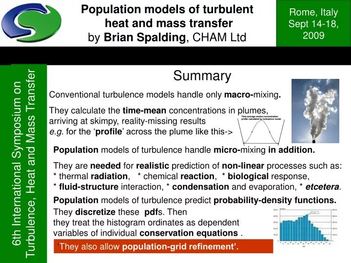
Population models of turbulent heat and mass transfer by Brian Spalding , CHAM Ltd. Summary. Conventional turbulence models handle only macro- mixing . They calculate the time-mean concentrations in plumes, arriving at skimpy, reality-missing results

E N D
Population models of turbulent heat and mass transfer by Brian Spalding, CHAM Ltd Summary Conventional turbulence models handle only macro-mixing. They calculate the time-mean concentrations in plumes, arriving at skimpy, reality-missing results e.g. for the ‘profile’ across the plume like this-> Population models of turbulence handle micro-mixing in addition. They are needed for realistic prediction of non-linear processes such as: * thermal radiation, * chemical reaction, * biological response, * fluid-structure interaction, * condensation and evaporation, * etcetera. Population models of turbulence predict probability-density functions. They discretize these pdfs. Then they treat the histogram ordinates as dependent variables of individual conservation equations . ‘They also allow population-grid refinement’.
Population models of turbulent heat and mass transfer; how turbulent mixing proceeds Boussinesq’s enlarged-viscosity concept predicts macro-mixing well, but not micro-mixing. It is eddy roll-up, enlarging interface areas and concentration gradients, which allows laminar diffusion to do its work. On the left is Urban Svenson’s 1998 numerical simulation of the Kelvin-Hemholtz instability which causes eddy roll-up. The probability-density function for this location will look like this: On the right is a sketch of the 1970’s ‘ESCIMO’ concept of how ‘Engulfment’ and ‘Stretching’ increase gradients of temperature and concentration and so facilitate chemical reaction (Noseir, 1980).
Population models of turbulent heat and mass transfer; fundamental concepts • In what follows, transient engulfment and stretching processes are postulated as occurring continually and throughout the turbulent fluid. • They can be likened to ‘brief encounters’ between unlike parents, leading to offspring of intermediate complexion, as illustrated here: • In the absence of other guidance, the rate of offspring production is taken as proportional to the parent-concentration product, times: • the square root of the sum of products of velocity gradients. • This square root, multiplied by the effective viscosity, represents the • generation rate of turbulent kinetic energy, • linking conveniently with hydrodynamic turbulence models e.g. k-epsilon. • The pdf’s (now also called population distribution functions) of complexion are then computed via simple mass balances.
Population models of turbulent heat and mass transfer; some history • The use of mass-balance (I.e. ‘pdf-transport’) equations for computing population distributions was proposed by Dopazo in 1975. • Numerical solutions were first provided in 1981 by Pope, who (wisely?) chose the Monte-Carlo method for doing so. • Computations by Fueyo (2008) for hydrocarbon combustion, shown here, were also obtained by the Monte-Carlo method. • In 1996, independently and as a generalisation of the 1971 ‘eddy-break-up’ concept, I created the ‘multi-fluid model’. • This discretized the pdf, treating the histogram ordinates as the dependent variables of a sufficient number of differential equations. • Both 1D and 2D histograms were used; and attention was given to how many distinct ‘fluids’ (I.e. histogram ordinates) were required for for accuracy. This population-grid-refinement possibility, not available in the Monte Carlo method, is an advantage of the discretized approach.
Population models of turbulent heat and mass transfer; questions which research could answer. • The ‘offspring-production-rate’ equation contains a proportionality constant (CONMIX below) which must be obtained from experiment. • What is its value? • Is it indeed a constant? • If not, does it depend on Reynolds Number? on energy-dissipation/production-rate ratio? on something else? 2. Are ‘complexions’ of the offspring distributed In uniform ‘Mendelian’ fashion shown on the right)? Or is there just one offspring complexion, as shown on the left? 3. Pdf’s of temperature are easy to measure; and their shapes depend on the assumptions made for CONMIX and offspring distributions. Therefore the research questions can be answered, by comparing with experimental contour and pdf shapes and sizes (see next slides). 4. Unfortunately few researchers practise both experimental and numerical studies. How to change that is the most pressing research challenge.
Population models of turbulent heat and mass transfer; numerical solutions of the conservation equations Results will be presented for the much-studied steady axi-symmetrical uniform-density turbulent jet. • The macro-mixing part of the model is conventional in that: • the k-epsilon model is employed for the calculation of the effective viscosity; and • a constant effective Prandtl number characterises the turbulent diffusion of each of the hypothetically distinct fluids. • The micro-mixing part of the model is unconventional, in that: • each equation has a source term which expresses its rate of creation by the evening out of the steep concentration gradients within the engulfed eddy; and • it has a corresponding sink term expressing its contributions, with partnering ‘parents’, to new engulfments. If this mingling of disparate elements is adjudged inconsistent, so be it. Consistency is not always a virtue.
Population models of turbulence; fluid-concentration contours for a steady axi-symmetrical jet with CONMIX=100 Numerical simulation with a 20-fluid model and a 20*100 spatial grid leads to concentration contours of each fluid, e.g. : 1. Sum of all 20 fluids, I.e. the conventional mixture fraction 2. Fluid 1, of highest injected-substance concentration 3. Fluid 10, of smaller injected-substance concentration 4. Fluid 15, of still smaller injected-substance concentration 5. Fluid 20, of smallest injected-substance concentration Note that 20 additional differential equations had to be solved!
Population models of turbulence; fluid-concentration contours for the jet, with CONMIX=1 and 100 compared With CONMIX=1 (on the left) the contours are much broader than with CONMIX=100 (on the right, as just seen). Which are the more realistic? The ‘true’ value of CONMIX can be established by comparison of experimentally-measure pdf’s with calculated ones (see next slide). Fluid number: 1 10 15 20
Population models of turbulence; pdf’s at two points on the jet axis, for CONMIX=1, 10 and 100 Computed pdf’s for CONMIX = 1.0 10.0 and 100.0 Axial distance nozzle diameter = 10 Axial distance nozzle diameter = 18 Such large shape differences should make it easy to determine CONMIX
Population models of turbulent heat and mass transfer; population-grid-refinement effects Perhaps the 20-fluid model gives insufficient resolution of the pdf; therefore it is instructive to vary the ‘population-grid’ fineness, as shown below, for CONMIX= 5, for a point on the axis far from the nozzle. Number of fluids = 10 = 20 = 40 Number of fluids = 60 = 80 = 100
Population models of turbulent heat and mass transfer; comments on the foregoing results 1. Increasing the number of fluids does give the expected smoothing of the pdf shape; and it of course increases the computer time also. 2. Computer times are however very small (less than 1 PC minute). 3. The program was PHOENICS, which has a built-in (but user- adjustable) multi-fluid model and a library of input files. 4. What is now needed is that experimental researchers should use it, or some equivalent software. 5. It is also desirable that Direct Numerical Simulation (DNS) practitioners should post-process their results in terms of pdf’s and of the quantitative conditions which influence them. 6. Aiding turbulence modellers in this way may be regarded as the main useful result which can emerge from DNS studies, until computing power increases greatly. 7. But the modellers need to abandon conventional Kolmogorov-type models and “think pdf”.
Population models of turbulent heat and mass transfer; three practical reasons for computing pdf’s 1. Death can be caused by breathing occasional whiffs of high-concentration poison-gas, the time-average concentration of which may be non-lethal. 2. It is the occasional high-velocity gust which damages the wind turbine, not the time-average wind force. 3. Explosions can still occur when onlysome pockets of mixture are in theflammable range of air-fuel ratios, even though the mixture as a whole is too rich or too lean to burn. It is differences from the mean which count !
Population models of turbulent heat and mass transfer; final remarks Four commonmisconceptions have been challenged, namely: 1. That turbulence models must be of Kolmogorov type, concerned only with mixture-average quantities, e.g. k, epsilon, RMS fluctuations, etc., perhapswith presumed pdf shapes. In fact, the pdfs of any fluid attribute (or pair of attributes) can be computed directly, with few and testable assumptions. 2. That Monte-Carlo methods must be used for computing pdfs. In fact, discretization issimpler (to understand and to program), and more informative; moreover it allows population-grid refinement studies. 3. That CFD has at most4 dimensions (3 of space and 1 of time). In fact, it must become multi-dimensional ifthe population-related aspects of fluids are to be simulated 4. That turbulence modelling is a unique activity, unlike any other. In fact, it is just one branch of population modelling, of which other branches concern: particle-size variation, bacterial growth and decay, animal-species interaction, etcetera.
Population models of turbulent heat and mass transfer Thank you for your attention! The End