Download
1 / 34
340 likes | 464 Views
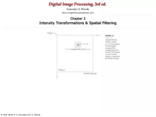
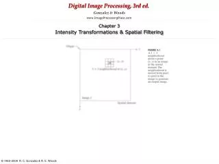
The spatial domain processes discussed in this chapter are denoted by the expression g(x,y)=T[f(x,y)] Where f(x,y) is the input image, g(x,y) is the output (processed) image, and T is an operator on f, defined over a specified neighborhood about point (x,y)

E N D
The spatial domain processes discussed in this chapter are denoted by the expression g(x,y)=T[f(x,y)] Where f(x,y) is the input image, g(x,y) is the output (processed) image, and T is an operator on f, defined over a specified neighborhood about point (x,y) Intensity transformation functions frequently are written in simplified form as s=T(r) Where r denotes the intensity of f and s the intensity of g, both at any corresponding point (x,y)
Function imadjust: Function imadjust is the basic IPT tool for intensity transformations of gray scale images. It has the syntax g=imadjust(f, [low_in high_in], [low_out high_out], gamma)
Negative image, obtained using the command >>g1=imadjust(f,[0,1],[1,0]); This process, which is the digital equivalent of obtaining a photographic negative, is particularly useful for enhancing white or gray detail embedded in a large, predominantly dark region.
The negative of an image can be obtained also with IPT function imcomplement >> g=imcomplement(f) Expanding the gray scale region between 0.5 and 0.75 to the full [0,1] range: >> g2=imadjust(f,[0.5 0.75], [0 1]); This type of processing is useful for highlighting an intensity band of interest. >> g3=imadjust(f,[ ],[ ],2); produces a similar result by compressing the low end and expanding the high end of the gray scale.
Logarithmic Transformation: Logarithmic transformations are implemented using the expression g= c*log(1+double(f)) where c is a constant. The shape of this transformation is similar to the gamma curve with the low values set at 0 and the high values set to 1 on both scales. Note, however, that the shape of gamma curve is variable, whereas the shape of the log function is fixed. mat2gray(g) function brings the values to the range [0,1] im2uint8 brings them to the range [0, 255] g=im2uint8(mat2gray(log(1+double(f))); imshow(g)
Bit-plane slicing : Pixels are digital numbers composed of bits. For example, the intensity of each pixel in an 256-level gray-scale image is composed of 8 bits(i.e., one byte). Instead of highlighting intensity-level ranges, we could highlight the contributionmade to total image appearance by specific bits.
The histogram of a digital image with intensity levels in the range [0, L-1] is a discrete function h(rk)=nk Where rk is the kth intensity value and nk is the number of pixels in the image with intensity rk. It is common practice to normalize to normalize a histogram by dividing each of its components by the total number of pixels in the image, denoted by the product MN, where, as usual, M and N are row and column dimensions of the image.
Histogram Equalization is implemented in the toolbox by function histeq, which has the syntax g=histeq(f,nlev) where f is the input image and nlev is the number of intensity levels specified for the output image. Default value is nlev=64