Download
1 / 21
210 likes | 299 Views
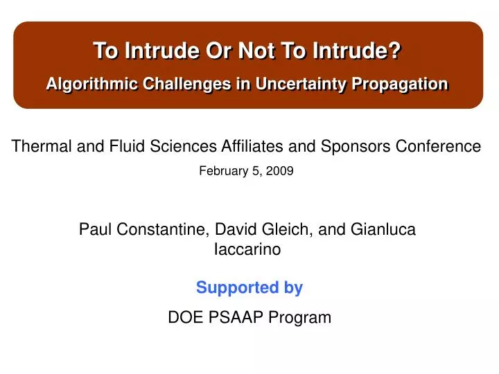
To Intrude Or Not To Intrude? Algorithmic Challenges in Uncertainty Propagation. Thermal and Fluid Sciences Affiliates and Sponsors Conference February 5, 2009. Paul Constantine, David Gleich, and Gianluca Iaccarino. Supported by DOE PSAAP Program. Input uncertainty. Output uncertainty.

E N D
To Intrude Or Not To Intrude? Algorithmic Challenges in Uncertainty Propagation Thermal and Fluid Sciences Affiliates and Sponsors Conference February 5, 2009 Paul Constantine, David Gleich, and Gianluca Iaccarino Supported by DOE PSAAP Program
Input uncertainty Output uncertainty Data The Modeling Process 1 Reality 4 Qualification 2 Assimilation Validation Mathematical Model Prediction Coding QoI Verification Computational Model 3
The Modeling Process 1 Input uncertainty Reality 4 Qualification 2 Output uncertainty Data Assimilation Validation Mathematical Model Prediction Coding QoI Verification Computational Model 3
Redefining The Problem Assume you want to compute a temperature field… “Certain” introduce parameters y “Uncertain” T = T(x) T = T(x,y) Recall that the new parameters may represent uncertainties in measured input quantities, geometries, model parameters, boundary conditions, etc. This introduces a new parameter space for the quantity of interest (e.g. temperature).
What New Questions Can We Ask? You now may ask… What is the average temperature over the range of y at a point x? What is the variance of temperature at a point x? What is the probability that the temperature will remain within some critical threshold at a point x?
How Can We Compute These Statistics? • Monte Carlo Methods • Random sampling from the parameter space of y. • Non-intrusive, but slow convergence.
How Can We Compute These Statistics? • Monte Carlo Methods • Random sampling from the parameter space of y. • Non-intrusive, but slow convergence. • Interpolation (Stochastic Collocation) • Interpolate solution at quadrature points in y, and integrals are quadrature rules. • Non-intrusive and fast convergence, but aliasing error and curse of dimensionality.
How Can We Compute These Statistics? • Monte Carlo Methods • Random sampling from the parameter space of y. • Non-intrusive, but slow convergence. • Interpolation (Stochastic Collocation) • Interpolate solution at quadrature points in y, and integrals are quadrature rules. • Non-intrusive and fast convergence, but aliasing error and curse of dimensionality. • Projection (Polynomial Chaos) • Project the solution onto a polynomial basis of the parameter space. • Fast convergence and best approximation, but intrusive and curse of dimensionality.
How Can We Compute These Statistics? • Monte Carlo Methods • Random sampling from the parameter space of y. • Non-intrusive, but slow convergence. • Interpolation (Stochastic Collocation) • Interpolate solution at quadrature points in y, and integrals are quadrature rules. • Non-intrusive and fast convergence, but aliasing error and curse of dimensionality. • Projection (Polynomial Chaos) • Project the solution onto a polynomial basis of the parameter space. • Fast convergence and best approximation, but intrusive and curse of dimensionality. There are efficient alternatives to Monte Carlo!
A Simple Example Given the equation: Compute:
Challenges for Polynomial Approximation Methods • There are pressing challenges that keep the polynomial approximation methods from mainstream use despite their fast convergence properties.
Challenges for Polynomial Approximation Methods • There are pressing challenges that keep the polynomial approximation methods from mainstream use despite their fast convergence properties. • Scalability. (One large scale run for each quadrature point.)
Challenges for Polynomial Approximation Methods • There are pressing challenges that keep the polynomial approximation methods from mainstream use despite their fast convergence properties. • Scalability. (One large scale run for each quadrature point.) • Curse of dimensionality. (Exponential increase in cost.)
Challenges for Polynomial Approximation Methods • There are pressing challenges that keep the polynomial approximation methods from mainstream use despite their fast convergence properties. • Scalability. (One large scale run for each quadrature point.) • Curse of dimensionality. (Exponential increase in cost.) • Global approximations. (Discontinuities and singularities in y.)
Challenges for Polynomial Approximation Methods • There are pressing challenges that keep the polynomial approximation methods from mainstream use despite their fast convergence properties. • Scalability. (One large scale run for each quadrature point.) • Curse of dimensionality. (Exponential increase in cost.) • Global approximations. (Discontinuities and singularities in y.) • Biased estimates. (Hard to estimate error.)
Challenges for Polynomial Approximation Methods • There are pressing challenges that keep the polynomial approximation methods from mainstream use despite their fast convergence properties. • Scalability. (One large scale run for each quadrature point.) • Curse of dimensionality. (Exponential increase in cost.) • Global approximations. (Discontinuities and singularities in y.) • Biased estimates. (Hard to estimate error.) • Intrusive or Non-intrusive?
Addressing the Challenges(What We Have Been Doing) We have developed a way to compute the (best approximation) projection with a weakly intrusive implementation. Assume the discrete solution is computed via an appropriate matrix equation.
Addressing the Challenges(What We Have Been Doing) We have developed a way to compute the (best approximation) projection with a weakly intrusive implementation. Assume the discrete solution is computed via an appropriate matrix equation. Non-intrusive
Addressing the Challenges(What We Have Been Doing) We have developed a way to compute the (best approximation) projection with a weakly intrusive implementation. Assume the discrete solution is computed via an appropriate matrix equation. Non-intrusive Intrusive
Addressing the Challenges(What We Have Been Doing) We have developed a way to compute the (best approximation) projection with a weakly intrusive implementation. Assume the discrete solution is computed via an appropriate matrix equation. Weakly Intrusive Non-intrusive Intrusive
Take-home Message • There are efficient alternatives to Monte Carlo that are easy to implement and ready for use. • Stay tuned for reusable software libraries. Acknowledgements • We wish to acknowledge: • Generous support from the DOE ASC/PSAAP Program. • Valuable feedback and comments from the Stanford UQ Group. THANKS FOR YOUR ATTENTION!QUESTIONS?


![G3 - RADIO WAVE PROPAGATION [3 Exam Questions - 3 Groups]](https://cdn0.slideserve.com/484375/g3-radio-wave-propagation-3-exam-questions-3-groups-dt.jpg)


![G3 - RADIO WAVE PROPAGATION [3 Exam Questions - 3 Groups]](https://cdn1.slideserve.com/3333950/g3-radio-wave-propagation-3-exam-questions-3-groups-dt.jpg)