Download
1 / 63
670 likes | 892 Views
Interactive Segmentation. Oleg Kraz. “The human brain starts working the moment you are born and never stops until you stand up to speak in public ." George Jessel. Motivation. Manual segmentation is tedious and time consuming, lacking in precision.

E N D
Interactive Segmentation Oleg Kraz
“The human brain starts working the moment you are born and never stops until you stand up to speak in public." George Jessel
Motivation • Manual segmentation is tedious and time consuming, lacking in precision. • Fully automated segmentation is very difficult due enormous variety of images. • Solution: Semi-Automated segmentation. • Inteructive segmentation
what is interactive segmentation? • Automatic segmentation assisted with human “hints” for extracting objects from background. “hint” “hint”
Advantages • Quick and accurate • Intuitive and easy to use – just with a simple gesture of a mouse • Allows the user to edit the computed boundary and make changes, without starting from scratch.
Intelligent Scissors Definitions and reminders • Dijkstra's algorithm • Solves the single source (seed point) shortest path problem. Creates minimum cost spanning tree.
How does it work? The basic idea is to formulate the image as a weighted graph where pixels represent nodes with weighted edges connecting each pixel with its 8 adjacent neighbors. Wi
What are the waights? Image FeatureFormulation Laplacian Zero-Crossing fZ Gradient Magnitude fG Gradient Direction fD Since we are looking for “shortest paths”, this image features should describe the local costof transition from pixel a to b.
What are the waights? Image FeatureFormulation Laplacian Zero-Crossing fZ Gradient Magnitude fG Gradient Direction fD Since we are looking for “shortest paths”, this image features should describe the local costof transition from pixel a to b.
Local Costs If p and q are two neighboring pixels in the image then l(p, q) represents the local cost on the directed link (or edge) from p to q. The local cost function is a weighted sum of component cost functions. l(p,q) = ωZ • fZ(q) + ωG • fG(q) + ωD • fD (p,q) (Empirically, weights of ωZ= 0.43, ωD= 0.43, and ωG= 0.14 seem to work well in a wide range of images.)
Laplacian Zero-Crossing (fZ) Convolution with laplacian kernel approximates the 2nd partial derivative of the image
Laplacian Zero-Crossing (fZ) • Binary edge feature used for edge localization • Finds maximal (or minimal) gradient magnitude. • Laplacianzero-crossings represent “good” edge properties and should therefore have a low local cost.
Laplacian Zero-Crossing IL(q ) is the laplacian of an image Iat pixel q
Laplacian Zero-Crossing However, application of a discrete laplacian kernel to a digital image produces very few zero-valued pixels. The resulting feature cost contains wide cost “canyons” used for boundary localization. • Can be done with multiple kernel widths. smaller kernels are more sensitive to fine detail while larger kernels suppress noise
Laplacian Zero-Crossing With and withotlaplacian zero crossing:
Gradient Magnitude (fG) • Gradient magnitude - “Edge Strength” • Higher gradient magnitude - lower the cost. Thus gradient is scaled and inverted We can use multiple kernel sizes and choose the right for us (for every pixel)
Gradient Direction (fD) The gradient direction or orientation adds a smoothness constraint to the boundary by associating a relatively high cost for sharp changes in boundary direction.
Gradient Direction (fD) • D(p) - a unit vector of the gradient direction at a point p • D'(p) - the unit vector perpendicular (rotated 90° clockwise) to D(p) • L(p,q) is positive if the angle between D‘ (p) and the link (p,q) ≤ ) D’(p) D(p)
Gradient Direction (fD) The main purpose of including the neighborhood link direction is to associate a high cost with an edge between two neighboring pixels that have similar gradient directions but are perpendicular, or near perpendicular, to the link between them. Therefore, the direction feature cost is low when the gradient direction of the two neighboring pixels are similar to each other and the link between them
The algorithm • The graph search algorithm is initialized by placing a start or seed point, s, with a cumulative cost of 0, on an empty list, L (called the active list) • After initialization, the graph search then iteratively generates a minimum cost spanning tree of the image, based on the local function (Dijkstra+Nillson) • The active list is sorted with linear complexity
Example Example with gradient magnitude (for simplicity): Initial local cost map with the seed point circled
Example (cont.) Diagonal local costs have been scaled by Euclidean distance
Example (cont.) 47 points expanded
Example (cont.) Finished cumulative cost and path matrix with two of many paths
Interactive “Live-Wire” • Interactive movement of the free point by the mouse cursor causes the boundary to behave like a live-wire that follows the optimal path pointers from the free point back to the seed point • Seed point can be “snapped” to wanted edge by placing the mouse pointer close to the edge, using maximum gradient magnitude at specified neighborhood.
Path Cooling • More than two seed points are often required to accurately define an object’s boundary • many paths “coalesce” and share portions of their optimal path with other paths from other pixels • Using boundary cooling, seed points are automatically placed by finding a pixel on the active live-wire segment that has a “stable” history
Interactive Dynamic Training • On occasion, a section of the desired object boundary may have a weak gradient magnitude relative to a nearby strong gradient edge • Training exploits an object’s boundary segment that is already considered to be good and is performed dynamically as part of the boundary segmentation process.
Lazy snapping Interactive Image cutout tool - technique of removing an object from background. Foreground Background
Lazy snapping First, some reminder from a few weeks ago
cost function: • The cost function provides a soft constraint for segmentation and includes both region and boundary properties . • Let be a binary vector whose components can be either “obj” or “bkg” ,p the set of nods.
:Intuition • The can be seen as the individual penalties for assigning pixel p to “object” and “background” . • For example may reflect on how the intensity of pixel p fits into a known intensity model (e.g. histogram) of the object and background • comprises the “boundary” properties of segmentation A , Coefficient interpreted as a penalty for a discontinuity between p and q. • is large when pixels p and q are similar . • Costs may be based on local intensity gradient, Laplacian zero-crossing.
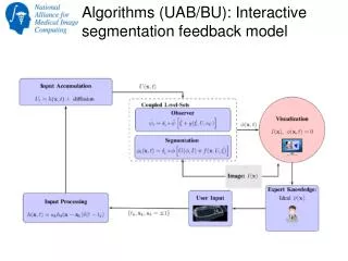
Implementation The general work : we create a graph with two terminals. The edge weights reflect the parameters in the regional and the boundary terms of the cost function, as well as the known positions of seeds in the image. The seeds are O = {v} and B = {p} Proceedings of “Internation Conference on Computer Vision”, Vancouver, Canada, July 2001
Lazy snapping • Consists of 2 steps: • Foreground and Background marking • Boundary editing
Lazy snapping • Suppose the image is a graph . • - Set of all pixels. • - Set of all arcs connecting adjacent nodes (4 or 8) We want to minimize the cost energy {foreground=1, background=0}