Download
1 / 35
360 likes | 485 Views
Intro to Excel 2010. What are the objectives of this session?. Familiarize you with spreadsheets and basic functions in Excel Apply certain mathematical manipulations to data ( u sing concepts introduced earlier in the course)

E N D
What are the objectives of this session? • Familiarize you with spreadsheets and basic functions in Excel • Apply certain mathematical manipulations to data (using concepts introduced earlier in the course) • Provide tools to make decisions and present data in effective ways
What is a Spreadsheet? • A computerized equivalent of a general ledger, where data are arranged in columns (vertical) and rows (horizontal) • A spreadsheet has several key uses: • Manipulating numerical data automatically by performing various user-defined calculations • Graphing data pointsfor visual analysis and presentation • Organizing and storing data, including non-numerical values
Starting Excel • Open All Programs under the Start Menu • Under the Microsoft Office folder select Microsoft Excel • Depending on your version of Windows, the wording and appearance may be slightly different
Minimize, Maximize, Close Excel Ribbon Help Button Minimize, Maximize, Close File File Menu (aka Backstage View) Sort/Filter Number Formats Formula Bar Columns Active Cell Fill Handle Rows Scroll Bars Tab Selector Mode Indicator (Change Views) Sheet Tabs New Sheet Zoom Slider
Cells, Sheets & Workbooks • Each cell has an address consisting of its column (letter) and row (number): A5orJ32 • Column is always listed first, followed by row • Cell address is used in referencing specific cells for formulas and charts • Cells can hold numbers, text, or formulas up to 32,000 characters in length! • Cells make up a Worksheet • 16,384 columns (lettered A-XFD) and 1,048,576 rows totaling 17,179,869,180 individual cells in each worksheet! • New files automatically contain 3 worksheets, named Sheet1, Sheet2 and Sheet3 • Sheets can be renamed (no spaces) by right-clicking on the sheet and selecting Rename • Workbooks are made up of worksheetsand are the same as the Excel File • Number of worksheets in a workbook is limited only by your computer’s memory but not recommended to have too many
Moving Around in Excel • The cells visible when a new worksheet opens are only a small portion of what is available for you to use. In order to move to areas that you cannot see, you can: • Use the scroll bars • Use the keys described below • Use the mouse • The Active Cell indicator (dark black border around a cell) tells you what cell you have selected
Excel Pointers • Hollow Plus • Used to select individual cells or cell range • Left Pointer • Appears when selecting menu options or buttons • Left Pointer with directional arrows • Appears when hovering over the bold black edge of selected cell(s) • Click and drag to move selection • Solid Plus • Appears when hovering over the fill handle on an active cell or cell range • Click and drag to use Fill command • Left-Right Arrow • Appears when hovering over the dividing line between columns • Click and slide left or right to adjust column width • Up-Down Arrow • Appears when hovering over the dividing line between rows • Click and slide up or down to adjust row height
Entering Data • Entering data is easy • Move the Active Cell indicator to the desired cell and begin typing • Activity 1: Enter the data from the following table into a new worksheet.
Editing Data • Several ways to edit data in cells • Double-click the cell you want to edit (cursor appears) • Select the cell you want to edit and hit the F2 button on the keyboard (cursor appears) • Using either method, you can edit directly in the cell or use the formula bar to modify cell contents • Activity 2: Edit three of the values in your table using any option above.
Deleting Data • To delete data • Select cell or cell range and hit <delete> key (<backspace> key will not work) • Select cell or cell range and use HomeEditingClearAll • Activity 3: Delete the last two values you have under “Apr” using either option above.
Undoing Edits • Undo button will undo recent changes • Activity 4: Undo the deletion you completed in Activity 3. The last two values you typed should appear again.
Columns and Rows • Cells default automatically to preset height and width • If cell values are too long to fit • Text displayed as ##### • Numbers displayed in scientific notation (2.3E+08) • Adjust column width with left-right arrow pointer, row height with up-down arrow pointer • Pointers appear when you hover between two rows or columns, click and slide to adjust OR double-click to automatically size to largest value • Right-click column or row, select Column Width or Row Height and enter desired value
Inserting & Deleting Cells • To insert a column, click on the column to the right of where you want to insert, then choose HomeCellsInsertInsert Sheet Columns • To insert a row, click on the row below where you want to insert, then choose HomeCellsInsertInsert Sheet Rows • To delete a row or column, highlight desired row or column, then choose HomeCellsDelete • To delete a cell or range of cells, select cell(s), then choose HomeCellsDeleteDelete cells • You will be prompted to choose how to adjust the sheet after deletion (move cells up, left, delete row, delete column) • Note: Inserting and Deleting cells, rows or columns may affect formulas or information in other cells
Activity 5: Insert/Delete • On your example spreadsheet, insert a column between Jun and Total; label the new column “Subtotal” • Insert a new row between Year B & Year C • Delete the CELL with the word “Subtotal”; when prompted, select “Shift cells left” • Delete the newly added row
Saving your Work • It is important to save your work as frequently as possible! • To save your workbook, click the Save button on the Quick Access toolbar (next to the Office Button) OR Select the Office Button, then Save or Save As • Activity 6: Save your worksheet to the computer desktop using a meaningful filename • Remember: • Excel suggests default file name “Book1” • Workbooks can have filenames up to 255 characters • The following characters are not allowed in file names: / \> < ? * | : ; • Use the “Save As” option if you want to save a copy of your file using a different filename or location
Close, Open Workbooks • Closing and Opening workbooks in Excel is the same as with other Microsoft Office software • Activity 7: Close the current workbook using the secondary Close button (below the close button for Excel) OR using the Office ButtonClose • Activity 8: Open your workbook by using Office ButtonOpen, then navigate to the fileyou just saved Close Excel Close File
Formatting • Formatting can be applied to numbers, text, cells and charts using various tools. • Number formats can be changed using HomeCellsFormatFormat Cells • Use the dialog box that appears to adjust how your numbers are displayed • Note: Changing number formats in Excel does NOT change the underlying numbers, only how they are displayed. Changing decimal places rounds the numbers accordingly. • Activity 9:Choose data values from your table and format them as desired.
Formulas & Functions • Excel provides many built-in functions to perform calculations with your data • Custom formulas can also be created • Click a blank cell where the formula result should appear. • Click FormulasInsert Function to show the Insert Function dialog box • You can search by function name or select a category to browse • Note: some functions have alternate versions with different parameters; a description of each function is listed at the bottom of the dialog box when you select it and be sure you are using the correct function.
Formulas & Functions (cont) • Once you select a function and click OK you will be taken to the Function Arguments dialog box to identify the range of cells and other variables required for the function to perform • Each argument required for the function selected will be described in the dialog box
Custom Formulas • Enter formulas directly into cells • All formulas must begin with an equals sign ( = ) • Use a blank cell to enter formulas • Remember order of operations (PEMDAS!) • Arithmetic operators in Excel • Addition: + • Subraction/Negation: - • Multiplication: * • Division: / • Exponents: ^ (eg: 3^2 = 32)
Reference Operators • Excel uses two ways to refer to cell combinations for calculations • Colon ( : ) – Range operator references all the cells in the range including the two references (eg: B5:B15 indicates B5, B6, B7…B15) • Comma ( , ) – Union operator combines multiple references into one (eg: =SUM(B5:B15,D5:D15) will sum all the cells between B5 and B15plus cells between D5 and D15)
Relative vs. Absolute References • Formulas can use cell references to identify values from a particular cell • Relative references – Excel will adjust the reference to the corresponding position when copied to a different cell • Absolute references – Excel will NOT adjust the reference to the corresponding position when copied to a different cell.
Relative vs. Absolute References (cont) • In this example, the conversion factor for miles to kilometers is entered in cell C1 • To calculate the conversion, cell B2 uses the formula (=A2*C1) • When the formula is copied to the cells below (B3:B5), the reference for the formula changes to (=A3*C2, =A4*C3, etc.) and produces the wrong result
Relative vs. Absolute References (cont) • To adjust the formula so that the conversion factor is used for all calculations you must use Absolute References • To force Excel to use the same reference for the formula in B2 has been changed to (=A2*$C$1) • When the formula is copied to the cells below (B3:B5), the reference for the formula stays the same (=A3*$C$1, =A4*$C$1, etc.) and produces the correct result
Relative vs. Absolute References (cont) • Absolute references can be used in three ways: • Fixed column: $A1 • Fixed row: A$1 • Fixed column and row: $A$1 • You can easily switch between relative and absolute references by selecting the cell with the reference and using the F4 key
Creating Charts • Charts can be used to graphically depict your data, emphasizing certain elements to help you make your point quickly and efficiently • Charts can be embedded into reports or presentations • Different charts are used for different purposes; it is important to make sure you use the correct chart for your data:
Creating Charts (cont) • Activity 10: Collect data from participant heights and enter it into a new worksheet. Select the cells with heights and create a chart (InsertCharts). Select an appropriate chart type (column, bar, line, scatter). • Using the participant heights data, create formulas to calculate the TOTAL, MIN, MAX, AVERAGE, MEDIAN, MODE, STDEV, and PERCENTILE
Creating Charts (cont) • Activity 11: Using your group’s data from the EPA Trends Report, create a data table in Excel. Create a chart using InsertCharts. • Excel creates an automatic chart for you; to edit or format components of the chart, select each item (either on the chart or under the Chart ToolsLayout tools) • Add/edit Chart title, Axis Titles, Legend, Data Labels, etc. • Under Chart ToolsFormat you can select various options to adjust colors, borders, etc.
Importing Text • Data from dataloggers or other equipment often produce text files • Various formats of text files can be imported into Excel (.txt, .csv, .xml, etc.) • Text files contain values that are either delimited (separated by specific characters such as a comma) or fixed-width (spaces between fields) • In a new blank worksheet, choose DataGet External DataFrom Text; the import text wizard appears and walks you through the steps to import the data
Printing • Before printing a worksheet it is recommended to preview first (PrintPrint Preview) • Print a worksheet using only a specified amount of pages (Office ButtonPrintPrintPreviewPage Setup, select “Fit to 1 page by 1 page” (Note: Excel will shrink all data in the print area to fit, but will not expand data if less than the pages needed are specified) • Adjust what data is printed or how it is printed by using other Page Layout options (Margins, Orientation, Print Area, etc.) • In Normal view, the spreadsheet will depict page breaks using vertical and horizontal dashed lines • Switch to Page Break Preview to adjust page breaks manually
Printing Titles • Excel can print headings or information in specified rows or columns on each page; this is useful when you have multiple pages of information • Page LayoutPrint Titles opens the Page Setup dialog box • Select or enter the cell range for the Rows to repeat at top or Columns to repeat at left as desired (ie. A1:K1) • If you want the Column or Row names (A, B, C and 1, 2, 3) to be displayed when printed, check the Row & Column Headings box
Fill & Series Commands • Use the Fill or Series Commands to let Excel enter data for you • Fill dates, number values, custom lists (auto fill only) • Select cells to fill (first cell must have starting value), then click HomeEditingFillSeries • OR, select first cell in series, grab Fill Handle, Right-click-and-drag to select cells to fill, select Series
Activity: Fill/Series • Using the table you created in Activity 1, practice using the Fill/Series command • Change “Year A” to “2012” • Select “2012” and the remaining “Year X” values • Click FillSeries, change the Type to Date, click OK • With the filled cells still selected, grab the fill handle and drag down several cells. Notice how the years continue to be filled in sequence
Custom Series • Fill custom series in two ways: • Enter first two values of series (ie. Year 1, Year 2) • Select both cells and drag fill handle to fill desired cells • Define custom list: Office ButtonExcelOptionsPopularEdit Custom Lists • Useful for text or mixed text/numeric values that are always in the same order (ie: FY12, FY13, etc.) • Select cells to be filled, with starting value in first cell then FillSeriesAutoFill OR select starting cell and drag fill handle to fill desired cells