Download

1 / 15
170 likes | 520 Views
The Primal-Dual Method: Steiner Forest. TexPoint fonts used in EMF. Read the TexPoint manual before you delete this box.: A A A A A A A A A A A A A. Network Design. Input: undirected graph G=(V,E) cost function: c:E ! R + connectivity requirements Output:

E N D
The Primal-Dual Method: Steiner Forest TexPoint fonts used in EMF. Read the TexPoint manual before you delete this box.: AAAAAAAAAAAAA
Network Design • Input: • undirected graph G=(V,E) • cost function: c:E ! R+ • connectivity requirements • Output: • minimum cost subgraph satisfying connectivity requirements • Example: • minimum spanning tree: minimum cost subgraph connecting all vertices
Steiner Tree • Input: • set of terminals T = {t1, …, tk} µ V • Output: • minimum cost subgraph connecting T • NP-complete • Algorithm: • define complete graph H on T • c(ti, tj) = shortest path in G from ti to tj • find a minimum spanning tree F in H • replace each edge in F by the corresponding path in G (delete cycles)
Steiner Tree: Analysis • F* - optimal Steiner tree in G • duplicate each edge in F* - all degrees are even • open up F* into a (Euler) cycle Z • c(Z) =2c(F*) • Z can be transformed into a spanning tree in H: • for any t,t’ 2 T: cZ(t,t’) ¸cH(t,t’) • Approximation factor = 2
Constrained Steiner Forest Problem • Input: • undirected graph G=(V,E) • cost function: c:E ! R+ • disjoint sets T1, … ,Tk ½ V • Output: • minimum cost subgraph H such that each set Ti belongs to a connected component of H S • Requirement function f: S ! {0,1} 8 S ½ V • f(S) =1 if there is a set Ti split between S and V-S • f(S) =0 otherwise • Note: f(S)=f(V-S), f is a function on cuts
Examples of Requirement Functions • Steiner tree: for any cut S separating terminals, f(S)=1 • shortest path between s and t: for any cut S separating s and t, f(S)=1 • minimum weight perfect matching: • f(S) =1 iff |S| is odd • (At least one vertex is matched outside S)
S δ(S) Linear Programming Formulation Covering LP Packing LP
Integrality Gap Example • Minimum spanning tree: all cuts are covered • Graph: cycle on n vertices, unit cost edges • Optimal integral solution: cost is n-1 • Optimal fractional solution: • for each edge e, x(e)=1/2 • all cuts are covered • cost is n/2 • Gap is 2-1/n
Primal-Dual Algorithm • y à 0 • AÃ; (x à 0) • While A is not a feasible solution • C - set of connected components S 2 (V,A) such that f(S)=1 • increase yS for all S 2 C until dual constraint for new e 2 E becomes tight • A à A [ {e} • Remove unnecessary edges from A
Primal-Dual Algorithm • y à 0 • AÃ; (x à 0) • While A is not a feasible solution • C - set of connected components S 2 (V,A) such that f(S)=1 • increase yS for all S 2 C until dual constraint for new e 2 E becomes tight • A à A [ {e} • Remove unnecessary edges from A • A’ – final solution
Analysis (1) Lemma: The primal solution generated by the algorithm satisfies the requirement constraints Proof: The `while’ loop continues till we get a feasible solution Lemma: The dual solution generated by the algorithm is feasible Proof: Whenever an edge becomes tight, no more cuts are “packed” into it
Analysis (2) Goal: charge the increase in primal cost in each iteration to the increase in dual cost Why is it important that we delete redundant edges at the end? Otherwise, we cannot charge tight primal edges to a single dual variable (the ball) – too many such edges!