Download
1 / 38
380 likes | 504 Views
Acknowledgment: Thomas Magnanti, Retsef Levi. Faster Primal-Dual Algorithms for the Economic Lot-Sizing Problem. Mihai Pătraşcu AT&T Research. Dan Stratila RUTCOR and Rutgers Business School Rutgers University. ISMP XX 25 August 2009. TexPoint fonts used in EMF.

E N D
Acknowledgment: Thomas Magnanti, Retsef Levi Faster Primal-Dual Algorithms for theEconomic Lot-Sizing Problem Mihai PătraşcuAT&T Research Dan StratilaRUTCOR and Rutgers Business SchoolRutgers University ISMP XX 25 August 2009 TexPoint fonts used in EMF. Read the TexPoint manual before you delete this box.: AAAAAAAAAAAAAA
Outline • Models: • The economic lot-sizing problem. • An important special case: the non-speculative condition. • Overview of previous results. • Review of “wave” primal-dual algorithm of Levi et al (2006). • Main result: a faster algorithm for the lot-sizing problem. • Conclusions: • Connection with basic algorithms problems. O(n)? • Wave primal-dual applicable to other inventory problems. ISMP XX
The Economic Lot-Sizing Problem ISMP XX
An Important Special Case ISMP XX
An Important Special Case ISMP XX
Outline • Models: • The economic lot-sizing problem. • An important special case: the non-speculative condition. • Overview of previous results. • Review of “wave” primal-dual algorithm of Levi et al (2006). • Main result: a faster algorithm for the lot-sizing problem. • Conclusions: • Connection with basic algorithms problems. O(n)? • Wave primal-dual applicable to other inventory problems. ISMP XX
Previous Results on Lot-Sizing Early research: • Introduced by Manne (’58), Wagner and Whitin (’58). • Wagner and Whitin (’58) provide O(n2) for non-speculative case. • Zabel (’64), Eppen et al (’69) obtain O(n2) for general case. • Results on heuristics, to be more efficient than O(n2) in ’70s-’80s. The O(n logn) algorithms: • Federgruen and Tzur (’91), forward algorithm. • Wagelmans et al (’92), backward algorithm, also relate to dual. • Aggarwal and Park (’93), using Monge arrays, generalizations. • These 3 algorithms run in O(n) for non-speculative case. Non-algorithmic results: • Krarup and Bilde (’77) show that above formulation is integral. • Polyhedral results for harder versions, e.g. multi-item lot-sizing: Production Planning by Mixed Integer Programming, Pochet and Wolsey (’06). ISMP XX
Primal-Dual Algorithms for Lot-Sizing Levi et al (’06) : • Obtain primal-dual algorithm for lot-sizing problem. • Proves above formulation is integral as a consequence. • Primal-dual 2-approxim. algorithms for joint replenishment problem (JRP), and for multistage assembly problem. • Algorithms clearly polynomial, authors do not estimate running times. Related primal-dual algorithms for facility location: • Primal-dual algorithms of Levi et al for inventory is rooted in primal-dual approximation algorithm for facility location of Jain and Vazirani (’01). • Thorup (’03) obtains 1.62 algorithm approximation algorithm for facility location with running time Õ(m+n) based on Jain and Vazirani (’01) and Jain et al (’03). Differences: • Algorithms for facility location and lot-sizing are different. • Input size is different: lot-sizing represented as facility would have O(n2) edges. ISMP XX
Outline • Models: • The economic lot-sizing problem. • An important special case: the non-speculative condition. • Overview of previous results. • Review of “wave” primal-dual algorithm of Levi et al (2006). • Main result: a faster algorithm for the lot-sizing problem. • Conclusions: • Connection with basic algorithms problems. O(n)? • Wave primal-dual applicable to other inventory problems. ISMP XX
Wave Primal-Dual Algorithm for Lot-Sizing (Modified, Levi et al ’06) ISMP XX
General • Start with (v,w)=0 and (x,y)=0 • Iteratively increase dual solution, increasing dual objective • At the same time, construct primal solution • When dual objective cannot be increased, primal is feasible • Post-processing step, O(n) • More details • To increase dual objective, we increase budgets vt • At some point, some of the constraints become tight • To keep increasing vt we begin increasing wst for those constraints • At some point some of the constraints become tight • Open s in the primal • Freeze all corresponding vt • Demands t with wst>0 assigned to order s • Remaining free choice—order in which vt are increased ISMP XX
The Wave • start increasing v4 • start increasing w44 • start increasing v3 • order 4 opens, budget 4 freezes demand 4 assigned to order 4 • start increasing w33 • start increasing v2 • start increasing w22 and w32 • order 2 opens, budgets 2 & 3 freeze demands 2 & 3 assigned to order 2 • start increasing v1 • start increasing w11 • order 1 opens, budgets 1 freezes, demand 1 assigned to order 1 • Types of events: • Demand point becomes active • Budget begins contributing to Kt • Order point becomes tight & assoc. ISMP XX
Wave Time and Position Wave time¿ Wave position W ISMP XX
Events: • Demand point becomes active • Budget begins contributing to Kt • Order point becomes tight & assoc. • Algorithms for digital computers: • Goal at end of execution to obtain • primal y and dual v. • Execute (3) from event to event, • instead of continuously • Step (3): • Compute wave position W* when • next order point becomes tight. • Update W:=W*, then updatevandw. ISMP XX
One iteration of (3): • For each unfrozen order point t, • compute position Wtwhen it becomes tight, • assuming no other unfrozen order points • become tight in the meantime. ISMP XX
One iteration of (3): • For each unfrozen order point t, • compute position Wtwhen it becomes tight, • assuming no other unfrozen order points • become tight in the meantime. • Compute W3 ISMP XX
One iteration of (3): • For each unfrozen order point t, • compute position Wtwhen it becomes tight, • assuming no other unfrozen order points • become tight in the meantime. • Compute W3 • Compute W2 ISMP XX
One iteration of (3): • For each unfrozen order point t, • compute position Wtwhen it becomes tight, • assuming no other unfrozen order points • become tight in the meantime. • Compute W3 • Compute W2 • Compute W1 ISMP XX
One iteration of (3): • For each unfrozen order point t, • compute position Wtwhen it becomes tight, • assuming no other unfrozen order points • become tight in the meantime. • Set W' = min{ Wt : t is unfrozen } Lemma:W' = W*, the position when the next order point becomes tight. Wtthat yields the minimum corresponds to the next order point that becomes tight. • Running time O(n3): • One computation of Wttakes O(n). • O(n) computations before an order point • becomes tight. • At most O(n) order points become tight. ISMP XX
One iteration of (3): • For each unfrozen order point t, • compute position Wtwhen it becomes tight, • assuming no other unfrozen order points • become tight in the meantime. • Set W' = min{ Wt : t is unfrozen } Lemma:W' = W*, the position when the next order point becomes tight. Wtthat yields the minimum corresponds to the next order point that becomes tight. • Running time O(n2): • With preprocessing Wttakes O(1) amortized. • O(n) computations before an order point • becomes tight. • At most O(n) order points become tight. ISMP XX
Outline • Models: • The economic lot-sizing problem. • An important special case: the non-speculative condition. • Overview of previous results. • Review of “wave” primal-dual algorithm of Levi et al (2006). • Main result: a faster algorithm for the lot-sizing problem. • Conclusions: • Connection with basic algorithms problems. O(n)? • Wave primal-dual applicable to other inventory problems. ISMP XX
Events: • Demand point becomes active • Budget begins contributing to Kt • Order point becomes tight & assoc • Algorithms for digital computers: • Goal at end of execution to obtain • primal y and dual v. • We will have “tentative” executions • of (3), which may be incorrect. • When we realize an execution is • incorrect, we go back and delete it. • Algorithm terminates => remaining • executions guaranteed correct. ISMP XX
Additional data structure: • Stack D = (ok, ok-1, …, o1) of • provisionally tight order points. • Stack initially empty, at end of loop (2) • will contain the correct order points. • Algorithm: • Start with D=(), t=n. • While t≥1: • 2.1) Compute time when order point tbecomes tight, taking into accountperiods t, …, n but ignoring periods 1, …, t-1. • 2.2) If t becomes tight before ok, delete ok from stack D, and go to 2.1. • 2.3) Add t to stack D, set t:=t-1. ISMP XX
t=3 • Additional data structure: • Stack D = (ok, ok-1, …, o1) of • provisionally tight order points. • Stack initially empty, at end of loop (2) • will contain the correct order points. • Algorithm: • Start with D=(), t=n. • While t≥1: • 2.1) Compute time when order point tbecomes tight, taking into accountperiods t, …, n but ignoring periods 1, …, t-1. • 2.2) If t becomes tight before ok, delete ok from stack D, and go to 2.1. • 2.3) Add t to stack D, set t:=t-1. ISMP XX
s2 e2 s3=e3 • Stack data structure: • Stack D = (ok, ok-1, …, o1) of • provisionally tight order points. • Stack initially empty, at end of loop (2) • will contain the correct order points. • Add information to stack: • E = ((ok, sk, ek), (ok-1, sk-1, ek-1), (o1,s1,e1) of • provisionally tight order points. • sk, …, ek are the demand points that were frozen when ok become tight. • Algorithm: • Start with D=(), t=n. • While t≥1: • 2.1) Compute time when order point tbecomes tight, taking into accountperiods t, …, n but ignoring periods 1, …, t-1. • 2.2) If t becomes tight before ok, delete ok from stack D, and go to 2.1. • 2.3) Add t to stack D, set t:=t-1. ISMP XX
s2 e2 s3=e3 • Stack data structure: • Stack D = (ok, ok-1, …, o1) of • provisionally tight order points. • Stack initially empty, at end of loop (2) • will contain the correct order points. • Add information to stack: • E = ((ok, sk, ek), (ok-1, sk-1, ek-1), …, (o1, s1, e1)) of provisionally tight order points. • sk, …, ek are the demand points that were frozen when ok became tight. • Algorithm: • Start with D=(), t=n. • While t≥1: • 2.1) Compute time when order point tbecomes tight, taking into accountperiods t, …, n but ignoring periods 1, …, t-1. • 2.2) If t becomes tight before ok, delete ok from stack D, and go to 2.1. • 2.3) Add t to stack D, set t:=t-1. • Add further information to stack: • E = ((ok, sk, ek, wk), (ok-1, sk-1, ek-1, wk), …, (o1,s1,e1,w1)) of provisionally tight order points. • wkis the wave position when ok became tight. ISMP XX
w4 • Stack data structure: • Stack D = (ok, ok-1, …, o1) of • provisionally tight order points. • Stack initially empty, at end of loop (2) • will contain the correct order points. • Add information to stack: • E = ((ok, sk, ek), (ok-1, sk-1, ek-1), …, (o1, s1, e1)) of provisionally tight order points. • sk, …, ek are the demand points that were frozen when ok became tight. • Algorithm: • Start with D=(), t=n. • While t≥1: • 2.1) Compute time when order point tbecomes tight, taking into accountperiods t, …, n but ignoring periods 1, …, t-1. • 2.2) If t becomes tight before ok, delete ok from stack D, and go to 2.1. • 2.3) Add t to stack D, set t:=t-1. • Add further information to stack: • E = ((ok, sk, ek, wk), (ok-1, sk-1, ek-1, wk), …, (o1,s1,e1,w1)) of provisionally tight order points. • wkis the wave position when ok became tight. ISMP XX
Stack data structure: • E = ((ok, sk, ek, wk), (ok-1, sk-1, ek-1, wk), …, (o1,s1,e1,w1)) of provisionally tight order points. • sk, …, ek are the demand points that were frozen when ok became tight. • wkis the wave position when ok became tight. • Algorithm details: • Once the wave position when tbecomes tight is computed, inserting the record into the stack takes O(1). • Deleting a record from the stack also takes O(1). • Every record is deleted at most once, and we make at most n insertions => at most O(n) deletions / computations / insertions. • Remains to do computation, in O(?) • Algorithm: • Start with E=(), t=n. • While t≥1: • 2.1) Compute time when order point tbecomes tight, taking into accountperiods t, …, n but ignoring periods 1, …, t-1. • 2.2) If t becomes tight before ok, delete ok from stack E, and go to 2.1. • 2.3) Add t to stack E, set t:=t-1. ISMP XX
Stack data structure: • E = ((ok, sk, ek, wk), (ok-1, sk-1, ek-1, wk), …, (o1,s1,e1,w1)) of provisionally tight order points. • sk, …, ek are the demand points that were frozen when ok became tight. • wkis the wave position when ok became tight. • Computation: • Define new set of numbers a1, …, an withat = ct + htn. • Only frozen demand points in segments sj,…,ej with at≤ h1n - wjcontribute to make order point t tight. • All unfrozen demand points in t, …, ok contribute. • Algorithm: • Start with E=(), t=n. • While t≥1: • 2.1) Compute time when order point tbecomes tight, taking into accountperiods t, …, n but ignoring periods 1, …, t-1. • 2.2) If t becomes tight before ok, delete ok from stack E, and go to 2.1. • 2.3) Add t to stack E, set t:=t-1. ISMP XX
w4 • Stack data structure: • E = ((ok, sk, ek, wk), (ok-1, sk-1, ek-1, wk), …, (o1,s1,e1,w1)) of provisionally tight order points. • sk, …, ek are the demand points that were frozen when ok became tight. • wkis the wave position when ok became tight. • Computation: • Define new set of numbers a1, …, an withat = ct + htn. • Only frozen demand points in segments sj,…,ej with at≤ h1n - wjcontribute to make order point t tight. • All unfrozen demand points in t, …, ok contribute. • Algorithm: • Start with E=(), t=n. • While t≥1: • 2.1) Compute time when order point tbecomes tight, taking into accountperiods t, …, n but ignoring periods 1, …, t-1. • 2.2) If t becomes tight before ok, delete ok from stack E, and go to 2.1. • 2.3) Add t to stack E, set t:=t-1. ISMP XX
w4 • Stack data structure: • E = ((ok, sk, ek, wk), (ok-1, sk-1, ek-1, wk), …, (o1,s1,e1,w1)) of provisionally tight order points. • sk, …, ek are the demand points that were frozen when ok became tight. • wkis the wave position when ok became tight. • Computation: • Define new set of numbers a1, …, an withat = ct + htn. • Only frozen demand points in segments sj,…,ej with at≤ h1n - wjcontribute to make order point t tight. • All unfrozen demand points in t, …, ok contribute. • Algorithm: • Start with E=(), t=n. • While t≥1: • 2.1) Compute time when order point tbecomes tight, taking into accountperiods t, …, n but ignoring periods 1, …, t-1. • 2.2) If t becomes tight before ok, delete ok from stack E, and go to 2.1. • 2.3) Add t to stack E, set t:=t-1. Key Lemma. Given min{ j : at≤ h1n – wj }, we candetermine in O(1) if order pointtbecomes tight beforeok. Iftbecomes tight afterok,we can compute inO(1) the wave position when t becomes tight. ISMP XX
w4 • Stack data structure: • E = ((ok, sk, ek, wk), (ok-1, sk-1, ek-1, wk), …, (o1,s1,e1,w1)) of provisionally tight order points. • sk, …, ek are the demand points that were frozen when ok became tight. • wkis the wave position when ok became tight. Key Lemma. Given j*= min{ j : at≤ h1n – wj }, we Can determine in O(1) if order pointtbecomes tight beforeok. Iftbecomes tight afterok,we can compute inO(1) the wave position when t becomes tight. Proof Idea. Can determine and perform the computation by inspecting each demand point in t, …, ok, and each record in k, …, j*. This would take O(n). Can perform in O(1), by computing the running sums d1, d1+d2, …, d1+d2+…+dn at start of algorithm, as well as certain running sums in the stack. Stack becomes E = ((ok, sk, ek, wk, Rk), (ok-1, sk-1, ek-1, wk, Rk-1), …, (o1,s1,e1,w1,R1)). • Algorithm: • Start with E=(), t=n. • While t≥1: • 2.1) Compute time when order point tbecomes tight, taking into accountperiods t, …, n but ignoring periods 1, …, t-1. • 2.2) If t becomes tight before ok, delete ok from stack E, and go to 2.1. • 2.3) Add t to stack E, set t:=t-1. ISMP XX
Time for Data Structures • Stack data structure: • E = ((ok, sk, ek, wk), (ok-1, sk-1, ek-1, wk), …, (o1,s1,e1,w1)) of provisionally tight order points. • sk, …, ek are the demand points that were frozen when ok became tight. • wkis the wave position when ok became tight. Key Lemma. Given j*= min{ j : at≤ h1n – wj }, we Can determine in O(1) if order pointtbecomes tight beforeok. Iftbecomes tight afterok,we can compute inO(1) the wave position when t becomes tight. Running time. O(n) iterations. Find j* using binary search in O(log(n)) Do the remaining computations in O(1) Total: O(n log n) • Algorithm: • Start with E=(), t=n. • While t≥1: • 2.1) Compute j* = min{ j : at ≤ h1n – wj }. • 2.2) Compute time when order point tbecomes tight, taking into accountperiods t, …, n but ignoring periods 1, …, t-1. • 2.2) If t becomes tight before ok, delete ok from stack E, and go to 2.1. • 2.3) Add t to stack E, set t:=t-1. Running time when non-speculative. O(n) iterations. Find j* in O(1), since a1, …, an are monotonic. Do the remaining computations in O(1) Total: O(n) Matches best times so far ISMP XX
Time for Data Structures • Stack data structure: • E = ((ok, sk, ek, wk), (ok-1, sk-1, ek-1, wk), …, (o1,s1,e1,w1)) of provisionally tight order points. • sk, …, ek are the demand points that were frozen when ok became tight. • wkis the wave position when ok became tight. Key Lemma. Given j*= min{ j : at≤ h1n – wj }, we Can determine in O(1) if order pointtbecomes tight beforeok. Iftbecomes tight afterok,we can compute inO(1) the wave position when t becomes tight. Improved running time. Machine: Word RAM 1) Sort a1, …, an in O(n log log n) before the start of the algorithm. 2) Create additional stack E’ that contains onlyn/log(n) entries out of the stack E. It divides E into buckets of size log(n). 3) Whenever a record is inserted into E’, look up the position of wk in a1, …, akand place it in the record. E’ = ((ok, sk, ek, wk, pk)). 4) When we have to find out j*, first look up in E’ using predecessor search, then look up in bucket in E using binary search. • Algorithm: • Start with E=(), t=n. • While t≥1: • 2.1) Compute j* = min{ j : at ≤ h1n – wj }. • 2.2) Compute time when order point tbecomes tight, taking into accountperiods t, …, n but ignoring periods 1, …, t-1. • 2.2) If t becomes tight before ok, delete ok from stack E, and go to 2.1. • 2.3) Add t to stack E, set t:=t-1. ISMP XX
Time for Data Structures • Stack data structure: • E = ((ok, sk, ek, wk), (ok-1, sk-1, ek-1, wk), …, (o1,s1,e1,w1)) of provisionally tight order points. • sk, …, ek are the demand points that were frozen when ok became tight. • wkis the wave position when ok became tight. • Improved running time. • Machine: Word RAM • 1) Sort a1, …, an in O(n log log n) before the start • of the algorithm. • 2) Create additional stack E’ that contains only • n/log(n) entries out of the stack E. It divides E into • buckets of size log(n). • 3) Whenever a record is inserted into E’, look up • the position of wk in a1, …, akand place it in the • record. E’ = ((ok, sk, ek, wk, pk)). • 4) When we have to find out j*, first look up in E’ • using predecessor search, then look up in bucket • in E using binary search. • Running time: • O(n log log n). • Each addition takes O(log(n)), there are O(n/log(n)) additions, for a total of O(n). [*] • Predecessor search takes O(log log n),O(n) lookups for a total of O(n log log n). • 4.1) Bucket size is O(log n), lookup takes O(log log n), total O(n log log n) • Algorithm: • Start with E=(), t=n. • While t≥1: • 2.1) Compute j* = min{ j : at ≤ h1n – wj }. • 2.2) Compute time when order point tbecomes tight, taking into accountperiods t, …, n but ignoring periods 1, …, t-1. • 2.2) If t becomes tight before ok, delete ok from stack E, and go to 2.1. • 2.3) Add t to stack E, set t:=t-1. Total: O(n log log n) ISMP XX
Conclusions • We obtain a O(n log log n) algorithm for lot-sizing, improving upon theO(n log n) results from 1991–1993. • We connect the lot-sizing problem to basic computing primitives—sorting and predecessor search. • Opportunity for further improvement in running time. • Opportunity for other insights. • Wave primal-dual algorithms run on other inventory problems (JRP, multi-stage assembly). • O(n+sort(n))? O(n)? ISMP XX