Download

1 / 45
450 likes | 507 Views
Normal Distribution. بسم الله الرحمن الرحیم. اردیبهشت 1390. Suppose we measured the right foot length of 30 persons and graphed the results. Assume the first person had a 10 inch foot. We could create a bar graph and plot that person on the graph.

E N D
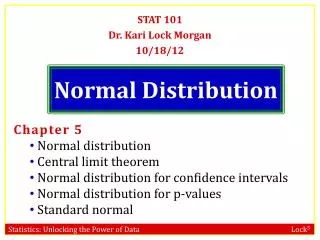
Normal Distribution بسم الله الرحمن الرحیم اردیبهشت 1390
Suppose we measured the right foot length of 30 persons and graphed the results. Assume the first person had a 10 inch foot. We could create a bar graph and plot that person on the graph. If our second subject had a 9 inch foot, we would add her to the graph. As we continued to plot foot lengths, a pattern would begin to emerge. 8 7 6 5 4 3 2 1 Number of People with that Shoe Size 4 5 6 7 8 9 10 11 12 13 14 Length of Right Foot Slide from Del Siegle
Notice how there are more people (n=6) with a 10 inch right foot than any other length. Notice also how as the length becomes larger or smaller, there are fewer and fewer people with that measurement. This is a characteristics of many variables that we measure. There is a tendency to have most measurements in the middle, and fewer as we approach the high and low extremes. If we were to connect the top of each bar, we would create a frequency polygon. 8 7 6 5 4 3 2 1 Number of People with that Shoe Size 4 5 6 7 8 9 10 11 12 13 14 Length of Right Foot Slide from Del Siegle
You will notice that if we smooth the lines, our data almost creates a bell shaped curve. 8 7 6 5 4 3 2 1 Number of People with that Shoe Size 4 5 6 7 8 9 10 11 12 13 14 Length of Right Foot Slide from Del Siegle
You will notice that if we smooth the lines, our data almost creates a bell shaped curve. This bell shaped curve is known as the “Bell Curve” or the “Normal Curve.” 8 7 6 5 4 3 2 1 Number of People with that Shoe Size 4 5 6 7 8 9 10 11 12 13 14 Length of Right Foot Slide from Del Siegle
n=16 n=4 n=8 n=512 n=256 n=64 n=32 n=128
9 8 7 6 5 4 3 2 1 Number of Students 12 13 14 15 16 17 18 19 20 21 22 Points on a Quiz Whenever you see a normal curve, you should imagine the bar graph within it. Slide from Del Siegle
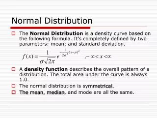
توزیع نرمال • این توزیع از نوع پیوسته است. • منحنی آن به شکل زنگوله ای و قرینه می باشد. • میانگین در آن با علامت μ نشان داده می شود. • انحراف معیار با حرف б نشان داده می شود. • میانگین و انحراف معیار دو پارامتر توزیع می باشند.
توزیع نرمال • مقدار μ ، محل دقیق میانگین را روی خط افقی مشخص می کند. • انحراف معیار ، б ، شکل توزیع را تعیین می کند. • تعداد منحنی های نرمال بسیارند و هریک دارای یک مقدارμ وб می باشند.
توزیع نرمال 68.2%
توزیع نرمال 68.2%
12+13+13+14+14+14+14+15+15+15+15+15+15+16+16+16+16+16+16+16+16+ 17+17+17+17+17+17+17+17+17+18+18+18+18+18+18+18+18+19+19+19+19+ 19+ 19+20+20+20+20+ 21+21+22 = 867 867 / 51 = 17 9 8 7 6 5 4 3 2 1 Number of Students 12 13 14 15 16 17 18 19 20 21 22 Points on a Quiz Now lets look at quiz scores for 51 students. The mean, Slide from Del Siegle
12 13 13 14 14 14 14 15 15 15 15 15 15 16 16 16 16 16 16 16 16 17 17 17 17 17 17 17 17 17 18 18 18 18 18 18 18 18 19 19 19 19 19 19 20 20 20 20 21 21 22 9 8 7 6 5 4 3 2 1 Number of Students 12 13 14 15 16 17 18 19 20 21 22 Points on a Quiz The mean, mode, Slide from Del Siegle
9 8 7 6 5 4 3 2 1 Number of Students 12 13 14 15 16 17 18 19 20 21 22 Points on a Quiz 12, 13, 13, 14, 14, 14, 14, 15, 15, 15, 15, 15, 15, 16, 16, 16, 16, 16, 16, 16, 16, 17, 17, 17, 17, 17, 17, 17, 17, 17, 18, 18, 18, 18, 18, 18, 18, 18, 19, 19, 19, 19, 19, 19, 20, 20, 20, 20, 21, 21, 22 will all fall on the same value in a normal distribution. The mean, mode, and median Slide from Del Siegle
خصوصیات توزیع نرمال • توزیع نرمال یک توزیع احتمالات است. • سطح زیر منحنی برابر با یک ( یا 100%) می باشد. • توزیع نرمال ، توزیع قرینه است. • نصف سطح زیر منحنی در طرف چپ خط قائمی که از میانگین می گذرد قرار دارد و نصف دیگر در طرف راست آن.
If your data fits a normal distribution, approximately 68% of your subjects will fall within one standard deviation of the mean. Slide from Del Siegle
If your data fits a normal distribution, approximately 68% of your subjects will fall within one standard deviation of the mean. Approximately 95% of your subjects will fall within two standard deviations of the mean. Slide from Del Siegle
If your data fits a normal distribution, approximately 68% of your subjects will fall within one standard deviation of the mean. Approximately 95% of your subjects will fall within two standard deviations of the mean. Over 99% of your subjects will fall within three standard deviations of the mean. Slide from Del Siegle
If your data fits a normal distribution, approximately 68% of your subjects will fall within one standard deviation of the mean. Approximately 95% of your subjects will fall within two standard deviations of the mean. Over 99% of your subjects will fall within three standard deviations of the mean.
On another test, a standard deviation may equal 5 points. If the mean were 45, then 68% of the students would score from 40 to 50 points. 30 35 40 45 50 55 60 Points on a Different Test The number of points that one standard deviations equals varies from distribution to distribution. On one math test, a standard deviation may be 7 points. If the mean were 45, then we would know that 68% of the students scored from 38 to 52. • 31 38 45 52 59 63 • Points on Math Test Slide from Del Siegle
Because the tail is on the negative (left) side of the graph, the distribution has a negative (left) skew. Data do not always form a normal distribution. When most of the scores are high, the distributions is not normal, but negatively (left) skewed. Skew refers to the tail of the distribution. 8 7 6 5 4 3 2 1 Number of People with that Shoe Size 4 5 6 7 8 9 10 11 12 13 14 Length of Right Foot Slide from Del Siegle
When most of the scores are low, the distributions is not normal, but positively (right) skewed. Because the tail is on the positive (right) side of the graph, the distribution has a positive (right) skew. 8 7 6 5 4 3 2 1 Number of People with that Shoe Size 4 5 6 7 8 9 10 11 12 13 14 Length of Right Foot Slide from Del Siegle
When data are skewed, they do not possess the characteristics of the normal curve (distribution). • For example, 68% of the subjects do not fall within one standard deviation above or below the mean. • The mean, mode, and median do not fall on the same score. • The mode will still be represented by the highest point of the distribution, but the mean will be toward the side with the tail and the median will fall between the mode and mean. Slide from Del Siegle
mean median mode mode median mean Negative or Left Skew Distribution Positive or Right Skew Distribution When data are skewed, they do not possess the characteristics of the normal curve (distribution). For example, 68% of the subjects do not fall within one standard deviation above or below the mean. The mean, mode, and median do not fall on the same score. The mode will still be represented by the highest point of the distribution, but the mean will be toward the side with the tail and the median will fall between the mode and mean. Slide from Del Siegle
توزیع نرمال استاندارد • توزیع نرمال که: • میانگین ، μ ، برابر با صفر باشد • انحراف معیار، б ، برابر با یک باشد • در مواقعی که میانگین یک توزیع نرمال برابر با صفر و انحراف معیار برابر با یک نمی باشد ؛ با تبدیل Z می توان براحتی از جدول نرمال استاندارد استفاده نمود.
Z Score (Standard Score) • Z = X - μ • مقدار نمره Z، تفاوت از میانگین در واحد انحراف معیار را بیان می نماید. • مقدار نمره Z، تا دو عدد اعشار محاسبه می گردد. σ
Tables • Areas under the standard normal curve (Appendices of the textbook)
تمرین • در نظر بگیرید ضربان قلب طبیعی در افراد سالم دارای توزیع نرمال بوده با میانگین 70 و انحراف معیار 10 ضربه در دقیقه (Mean = 70 and Standard Deviation =10 beats/min ) The exercises are modified from examples in Dawson-Saunders, B & Trapp, RG. Basic and Clinical Biostatistics, 2ndedition, 1994.
1 # تمرین بر این اساس: 1) چه بخشی از منحنی بالای 80 ضربه در دقیقه قرار می گیرد؟ Modified from Dawson-Saunders, B & Trapp, RG. Basic and Clinical Biostatistics, 2ndedition, 1994.
منحنی تمرین # 1 13.6% 2.14% 0.13% 15.9 % The exercises are modified from examples in Dawson-Saunders, B & Trapp, RG. Basic and Clinical Biostatistics, 2ndedition, 1994.
2 # تمرین 2) چه بخشی از منحنی بالای 90 ضربه در دقیقه قرار می گیرد؟ Modified from Dawson-Saunders, B & Trapp, RG. Basic and Clinical Biostatistics, 2ndedition, 1994.
منحنی تمرین # 2 2.14% 0.13% 2.3 % The exercises are modified from examples in Dawson-Saunders, B & Trapp, RG. Basic and Clinical Biostatistics, 2ndedition, 1994.
3 # تمرین 3) چه بخشی از منحنی بین 90 - 50 ضربه در دقیقه قرار می گیرد؟ Modified from Dawson-Saunders, B & Trapp, RG. Basic and Clinical Biostatistics, 2ndedition, 1994.
منحنی تمرین # 3 47.7% 47.7% 95.4 % The exercises are modified from examples in Dawson-Saunders, B & Trapp, RG. Basic and Clinical Biostatistics, 2ndedition, 1994.
4 # تمرین 4) چه بخشی از منحنی بالای 100 ضربه در دقیقه قرار می گیرد؟ Modified from Dawson-Saunders, B & Trapp, RG. Basic and Clinical Biostatistics, 2ndedition, 1994.
منحنی تمرین # 4 0.15% 0.15 % The exercises are modified from examples in Dawson-Saunders, B & Trapp, RG. Basic and Clinical Biostatistics, 2ndedition, 1994.
5 # تمرین 5) چه بخشی از منحنی کمتر از 40 ضربه در دقیقه یا بالای 100 ضربه در دقیقه قرار می گیرد؟ Modified from Dawson-Saunders, B & Trapp, RG. Basic and Clinical Biostatistics, 2ndedition, 1994.
منحنی تمرین # 5 0.15% 0.15% 0.3 % The exercises are modified from examples in Dawson-Saunders, B & Trapp, RG. Basic and Clinical Biostatistics, 2ndedition, 1994.
Solution/Answers 1) 15.9% or 0.159 2) 2.3% or 0.023 3) 95.4% or 0.954 4) 0.15 % or 0.0015 5) 0. 15 % or 0.0015 (for each tail) The exercises are modified from examples in Dawson-Saunders, B & Trapp, RG. Basic and Clinical Biostatistics, 2ndedition, 1994.
Application/Uses of Normal Distribution • It’s application goes beyond describing distributions • It is used by researchers and modelers. • The major use of normal distribution is the role it plays in statistical inference. • The z score along with the t –score, chi-square and F-statistics is important in hypothesis testing. • It helps managers/management make decisions.
6 # تمرین 6) اگر فشارخون سیستولیک در افراد سالم نرمال بطور طبیعی با میانگین 120 و انحراف معیار 10 میلی متر جیوه توزیع شده باشد: چه مقداری از فشار خون سیستولیک سطح زیر منحنی نرمال را به دو قسمت پایین 95% و بالای 5% تقسیم می کند؟
منحنی تمرین # 6 95% 5% The exercises are modified from examples in Dawson-Saunders, B & Trapp, RG. Basic and Clinical Biostatistics, 2ndedition, 1994.
پاسخ تمرین # 6 • Z = X - μ σ • با استفاده از جدول مقدار Z که مقادیر کمتر از 95% سطح زیر منحنی را از 5% بالایی سطح زیر منحنی جدا می کند، بدست می آوریم . 1.645=Z • 1.645 = X - 120 • 10))(1.645 ) = X - 120 10 • X = 136.45