Download
1 / 29
290 likes | 349 Views
AP Statistics Section 10.2 A CI for Population Mean When is Unknown .

E N D
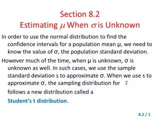
AP Statistics Section 10.2 ACI for Population Mean When is Unknown
It is extremely unlikely that we would actually know the standard deviation of a population. You should recall that this was one of the conditions necessary for us to construct a confidence interval for the population mean in section 10.1B.
In this section, we will discover how to construct a confidence interval for an unknown population mean when we don’t know the standard deviation . We will do this by estimating from the data.
The need to estimate changes some computational details of confidence intervals for but does not change their interpretation.
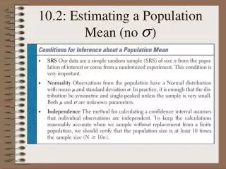
As before, we need to verify three important conditions before we estimate a population mean.
Our data are a SRS of size n from the population of interest or come from a randomized experiment. This condition is very important. If we do not have an SRS, our conclusions may not generalize to the population!!
Observations from the population have a Normal distribution with mean and standard deviation (both and are unknown). In practice, it is enough that the distribution be ____________ and _________________ unless the sample is very small. This will be discussed further in 10.2B
The method for calculating a confidence interval assumes that individual observations are independent. To keep the calculations reasonably accurate when we sample without replacement from a finite population, we should verify that the population size is at least ____ times the sample size (________).
In Chapter 9, we found that the sample mean, , has a Normal distribution with mean ___ and standard deviation ______. But, now we don’t know so weestimate it by the sample standard deviation s. So we now estimate the standard deviation of by _______,
When the standard deviation of a statistic is estimated from a sample, the result is called the____________ of the statistic.
When is used for the standard deviation of the distribution of instead of , the resulting distribution is no longer Normal.
Unlike the standard Normal distribution (or z-distribution), there is a different t distribution for each sample size n. We specify a particular t distribution by giving its degrees of freedom( df).
When we perform inference about using a t distribution, the appropriate degrees of freedom is df= ______. There are other t statistics with different degrees of freedom that we will encounter later. We will write the t distribution with k degrees of freedom as _____.
When the actual df does not appear in table B, use the largest df available that is less than your desired df.
The t distribution corresponding to any fixed number of degrees of freedom is _______________ and __________
Each t distribution is morespread out than the standard normal (z) distribution (i.e less concentrated about the mean).
As the degrees of freedom increase (i.e. the sample size increases), the spread of the corresponding t distribution decreases. In fact, as the degrees of freedom increase, the corresponding sequence of t distributions approaches the standard Normal ( z ) distribution. This happens because s estimates more accurately as the sample size increases.This is very important for us, because it allows us to continue to use the Central Limit Theorem.
Example: Suppose you want to construct a 95% confidence interval for the mean of a population based on an SRS of size 12. What critical value of t* should you use?
The one-sample t interval is similar in both reasoning and computational detail to the z interval in the previous section.
Draw an SRS of size n from a population having unknown mean . A level C confidence interval for is
Example: A number of groups are interested in studying the auto exhaust emissions produced by motor vehicles. Here is the amount of nitrogen oxides (NOX) emitted by light-duty engines (grams/mile) from a random sample of size n = 46. Construct and interpret a 95% confidence interval for the mean amount of NOX emitted by light-duty engines of this type.Remember to use the steps in the Inference Toolbox.
Parameter: The population of interest is ____________________. We want to estimate , the ____________________________.
Conditions: Since we do not know ____, use ______________________SRS:Normality:Independence: