Chapter 5. The Discrete Fourier Transform

1. Chapter 5. The Discrete Fourier Transform Gao Xinbo School of E.E., Xidian Univ. xbgao@ieee.org http://see.xidian.edu.cn/teach/matlabdsp/

2. Review 1 • The DTFT provides the frequency-domain (w) representation for absolutely summable sequences. • The z-transform provides a generalized frequency-domain (z) representation for arbitrary sequences. • Two features in common: • Defined for infinite-length sequences • Functions of continuous variable (w or z) • From the numerical computation viewpoint, these two features are troublesome because one has to evaluate infinite sums at uncountably infinite frequencies.

3. Review 2 • To use Matlab, we have to truncate sequences and then evaluate the expression at finitely many points. • The evaluation were obviously approximations to the exact calculations. • In other words, the DTFT and the z-transform are not numerically computable transform.

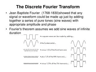
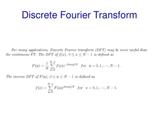
4. Introduction 1 • Therefore we turn our attention to a numerically computable transform. • It is obtained by sampling the DTFT transform in the frequency domain (or the z-transform on the unit circle). • We develop this transform by analyzing periodic sequences. • From FT analysis we know that a periodic function can always be represented by a linear combination of harmonically related complex exponentials (which is form of sampling). • This give us the Discrete Fourier Series representation. • We extend the DFS to finite-duration sequences, which leads to a new transform, called the Discrete Fourier Transform.

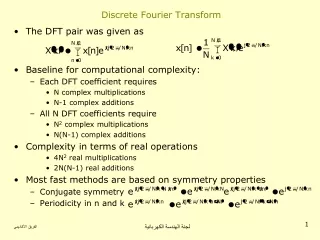
5. Introduction 2 • The DFT avoids the two problems mentioned above and is a numerically computable transform that is suitable for computer implementation. • The numerical computation of the DFT for long sequences is prohibitively time consuming. • Therefore several algorithms have been developed to efficiently compute the DFT. • These are collectively called fast Fourier transform (or FFT) algorithms.

6. The Discrete Fourier Series • Definition: Periodic sequence • N: the fundamental period of the sequences • From FT analysis we know that the periodic functions can be synthesized as a linear combination of complex exponentials whose frequencies are multiples (or harmonics) of the fundamental frequency (2pi/N). • From the frequency-domain periodicity of the DTFT, we conclude that there are a finite number of harmonics; the frequencies are {2pi/N*k,k=0,1,…,N-1}.

7. The Discrete Fourier Series • A periodic sequence can be expressed as are called the discrete Fourier series coefficients, which are given by The discrete Fourier series representation of periodic sequences

8. The Discrete Fourier Series • X(k) is itself a (complex-valued) periodic sequence with fundamental period equal to N. Example 5.1

9. Matlab Implementation Matrix-vector multiplication: Let x and X denote column vectors corresponding to the primary periods of sequences x(n) and X(k), respectively. Then DFS Matrix

10. dfs1 function(row vect.for dfs) • Function [Xk] = dfs (xn, N) • % Xk and xn are column(not row) vectors • if nargin < 2 N = length(xn) • n = 0: N-1; k = 0: N-1; • WN = exp(-j*2*pi/N); • kn = k’*n; • WNkn = WN.^kn; • Xk = WNkn * xn

11. Ex5.2 DFS of square wave seq. Note • Envelope like the sinc function; • Zeros occur at N/L (reciprocal of duty cycle); • Relation of N to density of freq. Samples;

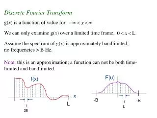
12. Relation to the z-transform The DFS X(k) represents N evenly spaced samples of the z-transform X(z) around the unit circle.

13. Relation to the DTFT The DFS is obtained by evenly sampling the DTFT at w1 intervals. The interval w1 is the sampling interval in the frequency domain. It is called frequency resolution because it tells us how close are the frequency samples.

14. Sampling and construction in the z-domain DFS & z-transform IDFS

15. Comments • When we sample X(z) on the unit circle, we obtain a periodic sequence in the time domain. • This sequence is a linear combination of the original x(n) and its infinite replicas, each shifted by multiples of N or –N. • If x(n)=0 for n<0 and n>=N, then there will be no overlap or aliasing in the time domain.

16. Comments RN(n) is called a rectangular window of length N. THEOREM1: Frequency Sampling If x(n) is time-limited (finite duration) to [0,N-1], then N samples of X(z) on the unit circle determine X(z) for all z.

17. Reconstruction Formula Let x(n) be time-limited to [0,N-1]. Then from Theorem 1 we should be able to recover the z-transform X(z) using its samples X~(k). WN-kN=1

18. The DTFT Interpolation Formula An interpolation polynomial This is the DTFT interpolation formula to reconstruct X(ejw) from its samples X~(k) Since , we have that X(ej2pik/N)=X~(k), which means that the interpolation is exact at sampling points.

19. The Discrete Fourier Transform • The discrete Fourier series provided us a mechanism for numerically computing the discrete-time Fourier transform. • It also alert us to a potential problem of aliasing in the time domain. • Mathematics dictates that the sampling of the discrete-time Fourier transform result in a periodic sequences x~(n). • But most of the signals in practice are not periodic. They are likely to be of finite duration.

20. The Discrete Fourier Transform • Theoretically, we can take care of this problem by defining a periodic signal whose primary shape is that of the finite duration signal and then using the DFS on this periodic signal. • Practically, we define a new transform called the Discrete Fourier Transform (DFT), which is the primary period of the DFS. • This DFT is the ultimate numerically computable Fourier transform for arbitrary finite duration sequences.

21. The Discrete Fourier Transform • First we define a finite-duration sequence x(n) that has N samples over 0<=n<=N as an N-point sequence The compact relationships between x(n) and x~(n) are The function rem(n,N) can be used to implement our modulo-N operation.

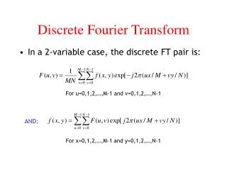
22. The Discrete Fourier Transform • The Discrete Fourier Transform of an N-point sequence is given by Note that the DFT X(k) is also an N-point sequence, that is, it is not defined outside of 0<=n<=N-1. DFT X(k) is the primary interval of X~(k).

23. Matlab Implementation

24. Examples 5.6 5.7 Comments • Zero-padding is an operation in which more zeros are appended to the original sequence. The resulting longer DFT provides closely spaced samples of the discrete-times Fourier transform of the original sequence. • The zero-padding gives us a high-density spectrum and provides a better displayed version for plotting. But it does not give us a high-resolution spectrum because no new information is added to the signal; only additional zeros are added in the data. • To get high-resolution spectrum, one has to obtain more data from the experiment or observations.

25. Properties of the DFT 1. Linearity: DFT[ax1(n)+bx2(n)]=aDFT[x1(n)]+bDFT[x2(n)] N3=max(N1,N2): N3-point DFT 2. Circular folding: Matlab: x=x(mod(-n,N)+1)

26. Properties of the DFT 3. Conjugation: 4. Symmetry properties for real sequences: Let x(n) be a real-valued N-point sequence

27. Comments: • Circular symmetry • Periodic conjugate symmetry • About 50% savings in computation as well as in storage. • X(0) is a real number: the DC frequency • X(N/2)(N is even) is also real-valued: Nyquist component • Circular-even and circular-odd components: Function, p143 The real-valued signals

28. Properties 5. Circular shift of a sequence 6. Circular shift in the frequency domain 7. Circular convolution**

29. Properties 8. Multiplication: 9. Parseval’s relation: Energy spectrum Power spectrum

30. Linear convolution using the DFT In general, the circular convolution is an aliased version of the linear convolution. If we make both x1(n) and x2(n) N=N1+N2-1 point sequences by padding an appropriate number of zeros, then the circular convolution is identical to the linear convolution.

31. Error Analysis • When N=max(N1,N2) is chosen for circular convolution, then the first (M-1) samples are in error, where M=min(N1,N2). n=0,1,…(N1+N2-1)-N X3(n) is also causal

32. Block Convolution • Segment the infinite-length input sequence into smaller sections (or blocks), process each section using the DFT, and finally assemble the output sequence from the outputs of each section. This procedure is called a block convolution operation. • Let us assume that the sequence x(n) is sectioned into N-point sequence and that the impulse response of the filter is an M-point sequence, where M<N. • We partition x(n) into sections, each overlapping with the previous one by exactly (M-1) samples, save at last (N-M+1) output samples, and finally concatenate these outputs into sequence. • To correct for the first (M-1) samples in the first output block, we set the first (M-1) samples in the first input blocks to zero.

33. Matlab Implementation Function [y]=ovrlpsav(x,h,N) Lenx = length(x); M=length(h); M1=M-1; L=N-M1; H = [h zeros(1,N-M)]; X = [zeros(1,M1), x, zeros(1,N-1); K = floor((Lenx+M1-1)/L); For k=0:K, xk = x(k*L+1:k*L+N); Y(k+1,: ) = circonvt(xk,h,N); end Y=Y(:,M:N)’; Y=(Y(:))’;

34. The Fast Fourier Transform • Although the DFT is computable transform, the straightforward implementation is very inefficient, especially when the sequence length N is large. • In 1965, Cooley and Tukey showed the a procedure to substantially reduce the amount of computations involved in the DFT. • This led to the explosion of applications of the DFT. • All these efficient algorithms are collectively known as fast Fourier transform (FFT) algorithms.

35. The FFT • Using the Matrix-vector multiplication to implement DFT: • X=WNx (WN: N*N, x: 1*N, X: 1*N) • takes N×N multiplications and (N-1)×N additions of complex number. Number of complex mult. CN=O(N2) • A complex multiplication requires 4 real multiplications and 2 real additions.

36. Goal of an Efficient computation • The total number of computations should be linear rather than quadratic with respect to N. • Most of the computations can be eliminated using the symmetry and periodicity properties CN=N×log2N If N=2^10, CN=will reduce to 1/100 times. Decimation-in-time: DIT-FFT, decimation-in-frequency: DIF-FFT

37. 4-point DFT→FFT example • X=Wx • X(0) = x(0)+x(2) + x(1)+x(3) = g1 + g2 • X(1) = x(0)-x(2) – j(x(1)-x(3)) = h1 - jh2 • X(2) = x(0)+x(2) - x(1)+x(3) = g1 - g2 • X(3) = x(0)-x(2) + j(x(1)-x(3)) = h1 + jh2 • It requires only 2 complex multiplications. • Signal flowgraph Efficient Approach

38. A 4-point DFT→FFT example

39. Divide-and-combine approach • To reduce the DFT computation’s quadratic dependence on N, one must choose a composite number N=LM since L2+M2<<N2 for large N. • Now divide the sequence into M smaller sequences of length L, take M smaller L-point DFTs, and combine these into a large DFT using L smaller M-point DFTs. This is the essence of the divide-and-combine approach.

40. Divide-and-combine approach Twiddle factor Three-step procedure: P155

41. Divide-and-combine approach • The total number of complex multiplications for this approach can now be given by • CN=ML2+N+LM2<o(N2) • This procedure can be further repeat if M or L are composite numbers. • When N=Rv, then such algorithms are called radix-R FFT algorithms.

42. A 8-point DFT→FFT example • 1. two 4-point DFT for m=1,2

44. Number of multiplications • A 4-point DFT is divided into two 2-point DFTs, with one intermedium matrix mult. • number of multiplications= 4×4cplx→ 2 ×1+ 1 ×4 cplx 16 →6 • A 8-point DFT is divided into two 4-point DFTs, with one intermedium matrix mult. • 8×8→2 ×6 + 2×4 64 →20 • For 16-point DFT: • 16×16→2 ×20 + 2×8 256 →56

45. In general the reduction of mult. • If N=M*L • N-pt DFT divided into • M times L-pt DFT + • Intermediate matrix transform + • L times M-pt DFT • CN=ML2+ML+LM2=N(M+L)<N2

46. Radix-2 FFT Algorithms • Let N=2v; then we choose M=2 and L=N/2 and divide x(n) into two N/2-point sequence. • This procedure can be repeated again and again. At each stage the sequences are decimated and the smaller DFTs combined. This decimation ands after v stages when we have N one-point sequences, which are also one-point DFTs. • The resulting procedure is called the decimation-in-time FFT (DIF-FFT) algorithm, for which the total number of complex multiplications is: CN=Nv= N*log2N; • using additional symmetries: CN=Nv= N/2*log2N • Signal flowgraph in Figure 5.19

47. function y=mditfft(x) • % 本程序对输入序列 x 实现时域抽取快速傅立叶变换DIT-FFT基2算法 • m=nextpow2(x); n=2^m; % 求x的长度对应的2的最低幂次m • if length(x)<n • x=[x,zeros(1,n-length(x))]; % 若x的长度不为2的幂次，补零到2的整数幂 • end • nxd=bin2dec(fliplr(dec2bin([1:n]-1,m)))+1; % 求1:2^m数列的倒序 • y=x(nxd); % 将x倒序排列得y的初始值 • for mm=1:m % 将DFT作m次基2分解,从左到右，对每次分解作DFT运算 • le=2^mm;u=1; % 旋转因子u初始化为w^0=1 • w=exp(-i*2*pi/le); % 设定本次分解的基本DFT因子w=exp(-i*2*pi/le) • for j=1:le/2 % 本次跨越间隔内的各次蝶形运算 • for k=j:le:n % 本次蝶形运算的跨越间隔为le=2^mm • kp=k+le/2; % 确定蝶形运算的对应单元下标 • t=y(kp)*u; % 蝶形运算的乘积项 • y(kp)=y(k)-t; % 蝶形运算 • y(k)=y(k)+t; % 蝶形运算 • end • u=u*w; % 修改旋转因子,多乘一个基本DFT因子w • end • end

48. Decimation-in-frequency FFT • In an alternate approach we choose L=2, M=N/2 and follow the steps in (5.49). • We can get the decimation-frequency FFT (DIF-FFT) algorithm. • Its signal flowgraph is a transposed structure of the DIT-FFT structure. • Its computational complexity is also equal to CN=Nv= N/2*log2N

49. Matlab Implementation • Function: X = fft(x,N) • If length(x)<N, x is padded with zeros. • If the argument N is omitted, N=length(x) • If x is matrix, fft computes the N-point DFT of each column of x • It is written in machine languag and not use the Matlab command. Therefore, it executes very fast. • It is written as a mixed-radix algorithm. • N=2v; N=prime number, it is reduced to the raw DFT.

50. Fast Convolutions • Use the circular convolution to implement the linear convolution and the FFT to implement the circular convolution. • The resulting algorithm is called a fast convolution algorithm. • If we choose N=2v and implement the radix-2 FFT, then the algorithm is called a high-speed convolution. • If x1(n) is N1-point, x2(n) is N2-point, then • Compare the linear convolution and the high-speed conv.