Download
1 / 45
450 likes | 631 Views
Solar Wind During the Maunder Minimum. Leif Svalgaard Stanford University Predictive Science, San Diego, 4 Sept. 2012. Indicators of Solar Activity. Sunspot Number (and Area, Magnetic Flux) Solar Radiation (TSI, UV, …, F10.7) Cosmic Ray Modulation Solar Wind Geomagnetic Variations

E N D
Solar Wind During the Maunder Minimum Leif Svalgaard Stanford University Predictive Science, San Diego, 4 Sept. 2012
Indicators of Solar Activity • Sunspot Number (and Area, Magnetic Flux) • Solar Radiation (TSI, UV, …, F10.7) • Cosmic Ray Modulation • Solar Wind • Geomagnetic Variations • Aurorae • Ionospheric Parameters • Climate? • More… Longest direct observations Rudolf Wolf After Eddy, 1976 Solar Activity is Magnetic Activity
Unfortunately Two Data Series Ken Schatten Hoyt & Schatten, GRL 21, 1994
How Well was the Maunder Minimum Observed? H&S It is not credible that for many years there were not a single day without observations Number of days per year with ‘observations’
More Realistic Assessment H&S 1825 1610 1700 Even after eliminating the spurious years with ‘no missing data’ there are enough left to establish that the Maunder Minimum had very few visible sunspots and was not due to general lack of observations 5% of 365 is ~20 days
The Ratio Group/Zurich SSN has Two Significant Discontinuities At ~1946 (after Max Waldmeier took over) and at ~1885 6
Locarno Effect of Weighting of Sunspots Sergio Cortesi Locarno is today the reference station of the official SIDC SSN SSN = 10*G+S In the 1940s the observers in Zürich [and Locarno] began to Weight spots. The net result is a ~20% inflation of the official Zürich SSN since ~1945 Unweighted count red
Compared with Sunspot Area (obs) Not linear relation, but a nice power law with slope 0.732. Use relation for pre-1945 to compute Rz from Area, and note that the observed Rz after 1945 is too high [by 21%]
Removing the discontinuity in ~1946, by multiplying Rz before 1946 by 1.20, yields Leaving one significant discrepancy ~1885 9
Wolf-Wolfer Groups Wolfer 80mm 64X Wolf 37mm 20X
Making a Composite Matched on this cycle Compare with group count from RGO [dashed line] and note its drift
Extending the Composite Comparing observers back in time [that overlap first our composite and then each other] one can extend the composite successively back to Schwabe: There is now no systematic difference between the Zurich SSN and a Group SSN constructed by not involving RGO.
K-Factors Why are these so different? 2% diff. No correlation
Why the large difference between Wolf and Wolfer? Because Wolf either could not see groups of Zurich classes A and B [with his small telescope] or deliberately omitted them when using the standard 80mm telescope. The A and B groups make up almost half of all groups
Removing the discontinuity in ~1885 by multiplying Rg by 1.47, yields Only two adjustments remove most of the disagreement and the evidence for a recent grand maximum (1945-1995)
The Effect on the Sunspot Curve SIDC No long-term trend the last 300 years
Removing the discrepancy between the Group Number and the Wolf Number removes the ‘background’ rise in reconstructed TSI I expect a strong reaction against ‘fixing’ the GSN from people that ‘explain’ climate change as a secular rise of TSI and other related solar variables
Some More TSI Reconstructions Kopp/LASP Crucial question: is there a slowly varying background? I think not.
The Auroral Record in Europe 45º 43º 51º 55º 60º 55º S. Sweden Hungary Denmark Effect of Changing Magnetic Latitude It is very difficult [impossible?] to calibrate accurately the auroral record because of the unknown ‘civilization’ correction.
80-110 Year ‘Gleissberg Cycle’ in Solar Activity Asymmetry? Extreme Asymmetry during the Maunder Minimum… There are various dynamo theoretical ‘explanations’ of N-S asymmetry. E.g. Pipin, 1999. I can’t judge these… Is this a ‘regular’ cycle or just over-interpretation of noisy data [like Waldmeier’s]? ‘Prediction’ from this: South will lead in cycle 25 or 26 and beyond. We shall see… Zolotova et al., 2010
How do we Know that the Poles Reversed Regularly before 1957? Wilcox & Scherrer, 1972 Svalgaard, 1977 The predominant polarity = polar field polarity (Rosenberg-Coleman effect) annually modulated by the B-angle. This effect combined with the Russell-McPherron effect [geomagnetic activity enhanced by the Southward Component of the HMF] predicts a 22-year cycle in geomagnetic activity synchronized with polar field reversals, as observed (now for 1840s-Present). “Thus, during last eight solar cycles magnetic field reversals have taken place each 11 year period”. S-M effect. Vokhmyanin & Ponyavin, 2012
Cosmic Ray Modulation Depends on the Sign of Solar Pole Polarity The shape of the modulation curve [alternating ‘peaks’ and ‘flat tops’] shows the polar field signs. North pole Ice cores contain a long record of 10Be atoms produced by cosmic rays. The record can be inverted to yield the cosmic ray intensity. The technique is not yetgood enough to show peaks and flats, but might with time be refined to allow this. North pole Svalgaard & Wilcox, 1976 Miyahara, 2011
The Cosmic Ray Record 17 pounds/yr 2 oz/year Steinhilber et al. 2012
24-hour running means of the Horizontal Component of the low- & mid-latitude geomagnetic field remove most of local time effects and leaves a Global imprint of the Ring Current [Van Allen Belts]: A quantitative measure of the effect can be formed as a series of the unsigned differences between consecutive days: The InterDiurnal Variability, IDV-index
IDV is strongly correlated with HMF B, but is blind to solar wind speed V
Space Climate Since we can reconstruct B, V, and n for 11 solar cycles we can determine an ‘average’ profile of the solar wind through the solar cycle
Solar Activity 1835-2011 Sunspot Number Ap Geomagnetic Index (mainly solar wind speed) Heliospheric Magnetic Field at Earth
Variation of ‘Open Flux’ Since we can also estimate solar wind speed from geomagnetic indices [Svalgaard & Cliver, JGR 2007] we can calculate the radial magnetic flux from the total B using the Parker Spiral formula: There seems to be both a Floor and a Ceiling and most importantly no long-term trend since the 1830s.
Floor and Ceiling of Solar Wind Alfvénic Mach number Ceiling Floor Observations seem to suggest that the magnitude of the solar cycle variation is invariant, i.e. does not depend on the size of the cycle. In particular, that the value at solar minimum is the same, ~12.25, in every cycle.
OMNI Explanation of MA Consider first the multi-species nature of the solar wind plasma: protons, alphas, electrons. We use subscripts p, a and e for these. N is density, T temperature, V flow speed, m mass Let Na = f*Np Ne = Np + 2*Na = Np*(1+2f) Mass density = mp*Np + ma*Na + me*Ne = mp*Np + 4*mp*f*Np = mp*Np * (1+4f) Thermal pressure = k * (Np*Tp + Na*Ta + Ne*Te) = k * (Np*Tp + f*Np*Ta + (1+2f)*Np*Te) = k*Np*Tp * [1 + (f*Ta/Tp) + (1+2f)*Te/Tp] Flow pressure = Np*mp*Vp**2 + Na*ma*Va**2 + Ne*me*Ve**2 = Np*mp*Vp**2 + f*Np*4*mp*Va**2 = Np*mp*Vp**2 * [l + 4f*(Va/Vp)**2] Rewrite: Mass density = C*mp*Np Thermal pressure = D*Np*k*Tp Flow pressure = E*Np*mp*Vp**2 Where C = 1+ 4f D = 1 + (f*Ta/Tp) + (1+2f)*Te/Tp E = 1 + 4f*(Va/Vp)**2 Now, some issues. 1. f is typically in the range 0.04-0.05, although there are significant differences for different flow types. 2. Ta/Tp is typically in the range 4-6. 3. What about Te? Feldman et al, JGR, 80, 4181, 1975 says that Te is almost always in the range 1-2*10**5 deg K. Te rises and falls with Tp, but with a much smaller range of variability. Kawano et al (JGR, 105, 7583, 2000) cites Newbury et al (JGR, 103, 9553, 1998) recommending Te = 1.4E5 based on 1978-82 ISEE 3 data. So we'll use Te = 1.4E5 deg K for our analysis. 4. What about (Va/Vp)**2? We should probably let this be unity always. If we let f=0.05, Ta=4*Tp, Va=Vp, and Te=1.4*10**5, we'd have C = 1.2 D = 1.2 + 1.54E5/Tp E = 1.2 Characteristic speeds: Sound speed = Vs = (gamma * thermal pressure / mass density)**0.5 = gamma**0.5 * [D*Np*k*Tp /C*mp*Np]**0.5 = gamma**0.5 * (D/C)**0.5 *(k*Tp/mp)**0.5 With the above assumptions for f, Ta, Va, and Te, and with gamma = 5/3, we'd get Vs (km/s) = 0.12 * [Tp (deg K) + 1.28*10**5]**0.5 Alfven speed = VA = B/(4pi*mass_density)**0.5 = B/(4pi*C*mp*Np)**0.5 With the above assumptions, we'd get VA (km/s) = 20 * B (nT)/Np**0.5 and MA = V/Va = (V * Np**0.5) / 20 * B
For MA = 7.5at all Maxima Question: Where would the MHD calculations fall in this diagram?
For MA = 12.25at all Minima MA =(V Np0.5)/(20 B) The marks the B = 4 nT contour of the ‘Floor’ in HMF
‘Burning Prairie’ => Magnetism Foukal & Eddy, Solar Phys. 2007, 245, 247-249
Deficit of Small Spots Large Small Lefevre & Clette, SIDC
The Livingston & Penn Data Temp. From 2001 to 2012 Livingston and Penn have measured field strength and brightness at the darkest position in umbrae of 1843 spots using the Zeeman splitting of the Fe 1564.8 nm line. Most observations are made in the morning [7h MST] when seeing is best. Livingston measures the absolute [true] field strength averaged over his [small: 2.5″x2.5″] spectrograph aperture, and not the Line-of-Sight [LOS] field.
Evolution of Distribution of Magnetic Field Strengths Sunspots form by assembly of smaller patches of magnetic flux. As more and more magnetic patches fall below 1500 G, fewer and fewer spots will form
We see fewer sunspots for given MPSI Calibration Change MWO Plage Strength Index Cycle variation and Trend ?
Working Hypothesis • The Maunder Minimum was not a deficit of magnetic flux, but • A lessening of the efficiency of the process that compacts magnetic fields into visible spots • This may now be happening again • If so, there is new solar physics to be learned