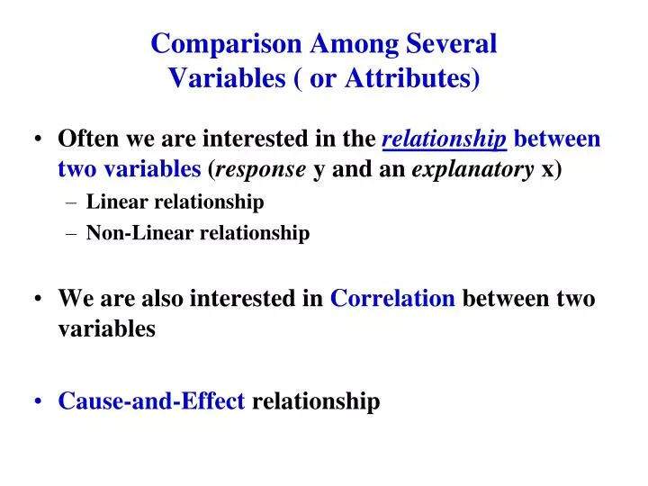
Comparison Among Several Variables ( or Attributes)

1. Comparison Among Several Variables ( or Attributes) • Often we are interested in the relationshipbetween two variables (response y and an explanatory x) • Linear relationship • Non-Linear relationship • We are also interested in Correlation between two variables • Cause-and-Effect relationship

2. Interpreting A Scatterplot . . Variable B . . . . Variables A and B show positive association . . . . . . . . . . . . . . . . . . . “Data in (a,b) form” . Variable A Definition : a) Two variables are positively associatedif (i) the above-average values of one tend to accompany the above-average values of the other and (ii) the below-average values tend to similarly occurtogether. b) They are negatively associated if the relationship is reversed

3. Linear Relationship • A straight line that describes the dependence of one variable, y, on the other variable, x, is called a regression line. • The equation for a straight line that depicts the relationship between variables y and x is expressed as : y = a + b ( x ) • where a is the intercept or value of y when x=0 • and b is the slope of the straight line

4. Least Square Regression Line Variable y . . . Minimize The deviation . . . Variable x The least square regression line is the line that makes thesum of the squares of the deviations of the data points from the line in the vertical direction as small as possible.

5. Least-Square Regression • Given a set of observed data (x1, y1), (x2,y2), - - - - (xn, yn) • Deviation = observed y - predicted y • Deviation = observed y - (a + bx) • ∑ (deviation**2) = ∑ [ (observed y – (a +bx)) **2 ] • Choose the a and b such that the SUM(deviation**2) is minimized • When the mathematics are worked out the Least-Square Regression Line is given by y = a + bx for n pairs of (x,y) where: b = [ ∑(xy) – (1/n)(∑ x)(∑y )] / [ ∑(x2) – (1/n)(∑ x)2 ] a= (mean y) - b * (mean x)

6. Least-Square Regression Line Example • (x,y) : ( 2,5), (3,7), (4,10), (5,13), (6,17), (7,19) • x : 2, 3, 4, 5, 6, 7 and ∑ (X ) = 27 • x**2 : 4, 9, 16, 25, 36, 49 and ∑ (X2) = 139 • y : 5, 7, 10, 13, 17, 19 and ∑ (Y) = 71 • xy : 10, 21, 40, 65, 102, 133 and ∑ (XY) = 371 • b = [371 – (1/6)(27)(71)] / (139) –(1/6)((27)**2) = 51.5 / 17.5 = 2.94 • a = (71/6) – ( 2.94 ) (27/6) = 11.8 – 13.23 = -1.43 • Least-Square Regression Line would be : y = - 1.43 + 2.94 x

7. Non-Linear Relationship • In the case of Linear relationship , for each equal increment of x, we “add” a fixed increment to arrive at y. • In Non-Linear relationship, for each equal increment of x, we may multiply or divide by an increment to arrive at y. • e.g. y = Ax + Bx**2 + C

8. Correlation • In the case of correlation we are looking at “association” which may NOT have the explanatory-response relationship. • Strength of association • Direction of association • We use a correlation coefficient, r, to measure the strength of linear association between two quantitative variables

9. Correlation Coefficient (Pearson) • Suppose we have n observations of 2 variables, x and y, which may not have the explanatory and responserelationships: (x1,y1), (x2,y2),--------, (xn, yn) Then the correlation coefficient, r, for variables x and y for these n cases may be computed as: r = (1/n-1) {∑ [((x-mean x)/std x) ((y – mean y)/std y)]} or a easier computational formula is r = [∑ (xy) –(1/n) (∑ x) (∑ y)]/[(n-1) (std x) (std y)] (for Pearson Correlation Coefficient)

10. Basic Properties of Correlation Coefficient, r • The value of r falls between –1 and 1 where a positive rindicates a positive association and a negative rindicates a negative association • The extreme values of r = -1 or r= 1 indicate that there is “perfect” linear association where the points in a scatter plot lie on a straight line. • The correlation coefficient r itself has no unit. So if the unit of measurement for x or for y or for both change, there is no effect on r. • Correlation coefficient only measures the strength & direction of the linear association between two variables

11. An Example of Correlation • Consider the situation where you are interested to see if program size and number of defects found during testing have any correlation. So you measured several programs. • (150 loc, 2 defects); (235, 3); (500, 4); (730, 7); (1000, 9) • Compute r via the equation • SUM (xy) = 18115 • 1/n = 1/5 = .2 • SUM x =2615 • SUM y = 25 • Numerator = 18115 - .2(2615)(25) = 5,040 • n-1 = 4 • Std x = 351 • Std y = 8.5 • Denominator = 4 (351)(8.5) = 11,934 • r = .42 • This r = .42 is pretty far from 1; so this set of data does not show strong correlation. But note what we can do with linear regression next. - assuming there is no computational mistakes (I think there may be some )

12. More about Least-Square Regression Line • Consider: • (x,y) : ( 150,2), (235,3), (500,4), (730,7), (1000,9) • x : 150, 235, 500, 730, 1000 and SUM (X ) = 2615 • x**2 : 26,250; 55,225; 250,000; 532,900; 1,000,000 and SUM (X**2) = 1,864,375 • y : 2, 3, 4, 7, 9 and SUM (Y) = 25 • xy : 300, 705, 2000, 5110, 9000 and SUM (XY) = 17,115 • B = [17115 – (1/5)(2615)(25)] / (1864375) –(1/5)((2615)**2) = 4040 / 496730 = .0081 • A = (25/5) – ( .0081 ) (2615/5) = 5 – 4.23 = .77 • Least-Square Regression Line would be : y = .77 + .0081 x

13. Try this Linear Equation • Y = .77 + .0081 X • put in the original number and see: • for x = 1000, y = .77 + 8.1 = 8.81 (close to 9) • for x = 500, y = .77 + 4.05 = 4.82 (close to 4) • for x = 150, y = .77 + 1.21 = 1.97 (close to 2) • try interpolate : • for x = 300, y = .77 + 2.43 = 3.2 (looks reasonable) • try extrapolate : • for x = 2000, y = .77 + 16.2 = 16.9 (this is not clear, besides there is nothing that says the linear relationship holds after x=1000.)

14. Spearman Rank Order correlation • We take the two sets of data Xi and Yi are converted to rankings of X’s and Y’s and the coefficient is computed using: r = 1 – [ (6*∑ (di )2 ) / n (n2 -1) ] where di = xi – yi (difference between ranking of x and y ) n = number of values in the each data set.

15. Consider a set of data points of (#of defect, loc) (7, 100); (6, 67); (8, 82); (9, 93) Example of Spearman’s Rank Order correlation Rank by defects Rank by size (diff)2 r = 1 –[ (6* (4+0+1+1)) / 4 (16-1) ] = 1 – (36/60) = .4 Not strong correlation ! (7,100) 1 4 3 (6,67) 4 4 0 (8,82) 2 1 3 (9,93) 1 1 2

16. Cause and Effect • Strong Correlation between two sets of measures alone does not mean “cause and effect” • For one measure to be the cause of another one must look at : • Sequence of occurrence • Cause must precede the consequence • Correlation • Two variables should be correlated • Logical deduction • Non-spurious relationship such as clothes length and stock market • Example: There is correct sequence and high correlation between coffee drinking programmers and very productive programmers; but the cause and effect of coffee is still questionable.