Download
1 / 25
250 likes | 394 Views
Periodic broadcasting with VBR-encoded video. Despina Saparilla , Keith W. Ross , and Martin Reisslein 1999 IEEE INFOCOM. Hsin-Hua, Lee. Objective.

E N D
Periodic broadcasting with VBR-encoded video Despina Saparilla, Keith W. Ross, and Martin Reisslein1999 IEEE INFOCOM Hsin-Hua, Lee
Objective • Develop non-uniform segmentation schemes with VBR-encoded video that significantly reduce the initial start-up latency without appreciably degrading image quality.
Introduction(1) • VoD (Video on Demand) • True VoD: client-centered • Arbitrary starting time • Waste of network bandwidth • Near VoD: data-centered • Utilization of network bandwidth and server capacity • Start-up latency • Batching the same requests before serving • Periodic Broadcasting
Introduction(2) • CBR (Constant Bit Rate) encoding technique • Modifying the quantization scale during compression • VBR (Variable Bit Rate) encoding technique • Quantization level remains constant • For the same quality level, Ave. Bit-RateCBR is typically 2 times or more the Ave. Bit-RateVBR • with VBR video there is potential for increased system efficiency Quality degradation Highly variable bit rate
Introduction(3) • To obtain dramatic reductions in start-up latency with VBR-encoded video, we must allow for some small fraction of packet loss (due to link buffer overflow). • Tradeoff between start-up latency and packet-loss. • Proposed Schemes • Bufferless multiplexing • Smoothing with bufferless multiplexing • Server-buffering • Client-prefetching
Near VoD with VBR-Encoded Video(1) • Notations
1 1 1 1 1 1 1 1 1 1 1 k 2 2 2 2 2 2 2 2 2 2 2 k k k k k k k k k k k 1 1 1 1 1 1 1 1 1 1 1 1 2 k 2 2 2 2 2 2 2 2 2 2 2 1 2 k k k k k k k k k k k k ˙ m*k m ˙ ˙ ˙ 1 1 1 1 1 1 1 1 1 1 1 1 2 k 2 2 2 2 2 2 2 2 2 2 2 1 2 k k k k k k k k k k k k 1 1 1 1 1 1 1 1 1 1 1 2 2 2 2 2 2 2 2 2 2 2 k k k k k k k k k k k Near VoD with VBR-Encoded Video(2)
Near VoD with VBR-Encoded Video(3) • Each video is divided into K segments according to broadcasting series. • General broadcasting series [e1,e2,…,eK-1,eK] • ei: the ith segment consists of ei segmentation units, in general, e1=1. • Ni(m): the number of frames in theithsegment of the mthvideo
Start-up latency vs. Loss Probability(1) • Loss of bits occurs when the aggregate bit rate of the traffic (i.e., from all MK streams) exceeds the link’s capacity, C.
Seg. 1 Seg. 2 Seg. 3 Seg. 4 Numerical Example: Geometric Series(1) Figure 1: Broadcasting strategy for geometric series with ek=2k-1. • q=K. • receiver storage is unlimited. • M=10, and N(m)=160,000 frames, about 107 mins. • F=25 frames/sec. • C: 85~205 Mbps.
Numerical Example: Geometric Series(3) • Two performance measures • Start-up latency • Probability of loss
K1 K2 K3 K4 Bufferless Statistical Multiplexing • Latency < 2 mins=> K at least 6 • Latency < 0.5 mins=> K at least 9 • As K increases, prob. of loss also becomes higher.
GoP Smoothing(1) • Total start-up latency = max. access time for 1st video segment + delay introduced due to smoothing over one GOP period. Figure 3: Bufferless multiplexing with smoothing over each GOP period
K=7 K=6 K=5 GoP Smoothing(2) • We refer to points that correspond to longer total start-up latencies with no further improvement in Ploss as dominated. • Smoothing over a higher number of GoP periods does not have an adverse effect when low start-up latencies are desirable. No significant effect ! Figure 4: Smoothing over many GOP periods (C=145M bps).
Buffered Statistical Multiplexing • Add in finite size buffer at the server link. • Total start-up latency = max. access time for 1st video segment + B/C. • To limit loss it is instead preferable to use a smaller K. K=7 K=6 K=5
virtual buffer Join-the-Shortest Queue Prefetching(1) server client prefetched frames client client prefetched buffer
Join-the-Shortest Queue Prefetching(2) • The JSQ prefetch policy attempts to balance the number of prefetched frames across all virtual buffers. • All the server needs to do is to schedule the broadcast of the frames of the MKvideo streams as if it were sending them to the MKdistinct virtual buffers.
C=145 Mbps Join-the-Shortest Queue Prefetching(3) • JSQ protocol brings significant improvement over simply multiplexing the video stream onto the bufferless link. 6 x 10⁻² 3 x 10⁻⁴ 6 x 10⁻⁸ 100.7 sec
Join-the-Shortest Queue Prefetching with prefetch delay(2) • dpre :the prefetch delay in frame periods. • Total start-up latency =(N1+dpre)/F C=145 MbpsK=7 3 x 10⁻⁴ 9 x 10⁻⁵ 6.6 x 10⁻⁶ 100.4 sec
VBR and CBR Compared • For the buffered multiplexing, we chose the K value and buffer size combination which gives the lowest delay while having a loss probability less than 10E-7 (essentially a negligible loss probability).