Download

1 / 60
600 likes | 782 Views
PISCO Progress. Carnegie A. Szentgyorgyi for A. Stark 20 March 2008. P arallel I mager for S outhern C osmology O bservations (PISCO): A Multiband Imager for Magellan. Antony Stark Smithsonian PI Christopher Stubbs Harvard PI Matt Holman Smithsonian — Planets, exoplanets

E N D
PISCO Progress Carnegie A. Szentgyorgyi for A. Stark 20 March 2008
Parallel Imager for Southern Cosmology Observations (PISCO):A Multiband Imager for Magellan • Antony Stark Smithsonian PI • Christopher Stubbs Harvard PI • Matt Holman Smithsonian — Planets, exoplanets • John Geary CCD electronics • Andy Szentgyorgyi Design consultant • Steve Amato CCD electronics • Michael Wood-Vasey Astronomer— Observing • Will High Thesis project, Harvard Physics • Andrea Loehr Astronomer — Observing algorithm • Brian StalderPostDoc, Harvard Physics • James Battat grad student, SAO • Armin Rest PostDoc— Photo-z Software • Steve Sansone LPPC machine shop
Dichroic in Cube Optical Layout Revised Optical Design of PISCO. Steve Schectman contributed to this design. The dichroics are embedded into cubes of fused silica, so that there is no difference in dielectric constant on either side of the dichroic. This allows the dichroics to be used at 45º. The dichroics are placed in the telecentric beam from the focal reducer, so all field positions have identical ranges of angle of incidence at the dichroics. The overall length of the instrument is reduced to 1.6 meters, and all CCDs are in a single, medium-sized dewar.
Current best desgin Design is 1.42 meters (56 inches) from focus to focus Design uses S-FPL51 glass
ADC Operation • Can use PISCO on Clay telescope • Consists of two rotating cylindrical prisms, • 1 cm thick • airspaced, multi-coated • Initial scientific mission can be achieved without ADC • ADC can be removed with re-focus
PISCO Design Concept Small Guider Housing Cable Wrap Shutter Dewar Wall ADC Dichroics & CCDs Lenses Electronics mounted here
Some Optics Have Been Ordered • Contract in place with Barr Associates for fabrication of Dichroic Cubes • This has a long lead time (8 months) and will drive the project timetable
Electronics are done… • We have already taken images in the lab with full control-to-image software. • Readout noise is OK (3 electrons). • Readout speed is OK ( < 8 seconds).
Initial detector tests look favorable Tested 2 3K x 6K 10 micron high-rho devices in Univ of Hawaii test system. Read noise Dark current vs. temperature CTE via Fe55 xrays Gain via Fe55 xrays
Analysis Software: We’ll build upon SuperMacho/ESSENCE image analysis pipeline Battle tested over past 6 years at CTIO for SM and ESSENCE surveys. Flatten with dome flats, fringe flat and sky flats Astrometric WCS registration, warp to fixed plate scale Photometry to 1% CVS code management, easy to add new modules Parallel implementation, Condor on Linux boxes Robust and self-tracking Honed on crowded fields Need to add (1) cluster photo-z module, and (2) SQL database Armin Rest, pipemeister, coming to CfA in Spring 2007.
Flow diagram for real-time cluster redshift analysis pipeline We expect that within 30 seconds of acquiring the first image, we will have produce an appraisal of whether the second 30 image will add enough integration time to obtain a cluster photometric redshift at the requisite SNR. We have in hand the middleware and pipeline structure for this, from the ESSENCE and SuperMacho surveys. We are missing only the final segment, namely the redshift estimator, which we will develop in parallel with the construction of the hardware.
Tightly coupled software/observing Take Image 1 30 sec Analyze Image: flatten, WCS, sextractor Galactic reddening corr. Produce z, sz OK? Offset Take Image 2 30 sec Offset if appropriate More images Slew to next target
Photometric Redshift for Clusters • Photo-z’s for individual galaxies tend to have scatter of sz/(1+z)~0.03, but with a few “catastrophic” outliers. • Combination of morphology, magnitude, color and location can be used to establish cluster’s redshift. • Robust statistics can be used to eliminate “outliers”.
Uniform exposure times for clusters Magnitudes in the four filter bands (shaded) for L*/2 early type galaxies, and exposure times (in seconds, unshaded) to achieve SNR=10, as a function of redshift. The table assumes galaxy flux integrated in a 2.2 arcsec diameter aperture, in seeing of 0.8 arcsec at an airmass of 1.2 in dark time. The numbers assume deep depletion detectors in the z and i bands, like those for the SMI. The exposure time needed to achieve SNR=10 is reasonably well matched across the bands. A minimum exposure time is 5 sec.
One night to obtain 115 cluster redshifts at z < 1.5 The time needed to obtain 115 cluster redshifts, in good conditions, is 8.2 hours. It will not be possible to obtain redshifts for the ~10% of clusters with redshift z > 1.5; these will be flagged to obtain redshifts using other instruments.
South Pole Telescope2007 First-Look Data • SPT data, Feb-April 2007 • 4 square degrees shown • red circles are known quasars • green regions are significant • negative regions in CMB: possible clusters • Current, upgraded SPT detector system shows two order of magnitude improvement in observing speed.
Magellan Observations of SPT Cluster Candidates LDSS3 multi-color photometry of SPT-selected region nr01
Abell 267, extrapolated to various redshifts and observed with PISCO
Order of detection by PISCO 8 bright red galaxies detected first (green circles) Black-circled detected next Blue dots are cluster galaxies Black dots are foreground
Histogram of photo-z of the first 18 galaxies and photo-z of the color-magnitude selected galaxies.
We are building the capability to efficiently chase SZ detections in optical • Blanco Cluster Survey (with Mohr et al) • Imaging with existing Magellan instruments • Spectroscopy with existing magellan instruments • Custom simultaneous multiband imager, PISCO
Ask a restricted set of questions • At a known position on the sky, is there a cluster of galaxies? • What is the redshift of the cluster? • We initially assume all galaxies are LRG’s • We make a redshift estimate based on this assumption • We use magnitude consistency to select the LRGs. • We then use a clustering algorithm to search for clustering in redshift space. • This is not the general problem of finding a photo-z for some random galaxy. • We are focusing on “luminous red galaxies”, LRG’s.
Why LRG’s? • These elliptical galaxies are preferentially found in custers, so they exhibit “clustering” more than, say, spirals. • They suffer minimal extinction/reddening due to dust in the galaxy, which can distort colors and therefore photo-z’s • They’re bright, and are crude standard candles, which helps in photo-z determination.
Photometric Redshift Principle The plots show how the observer-frame spectrum of a Luminous Red Galaxy (LRG) depends upon its redshift. The redshifts are indicated in the upper left corner of each panel. The flux ratios between the g, r, i, and z bands is a good indicator of galaxy redshift, as the 4000 Å break moves across the spectrum. We will develop real-time analysis code that will produce an initial cluster redshift result within 30 seconds of the acquisition of an image. From M. Blanton’s web page
Status of Observations • Reduction of BCS data under way • Flatfielding to better than 1% • Astrometric registration • Source Extractor photometry • Photo-z determination under development • Deep multiband images of initial SZ 2 degree region at (RA,DEC), plus similar region at arbitrary location for statistics • Long slit and muli-slit spectroscopy of selected galaxies in NR1 region • Additional nights both allocated & requested
Source Extractor Photometry • Used mag_auto fluxes from SE • Determine galaxy colors and uncertainties
A cluster photo-z estimator • Use Blanton’s K-correct code to predict SDSS colors for LRG vs. redshift. • Assume all galaxies are LRG’s • For each galaxy, for each trial redshift, compute error-weighted distance to prediction, for each color 4. Using distances for all 3 colors, calculate composite color distance vs. z 5. Pick z with minimum normalized color distance 6. Estimate redshift uncertainty by finding dz that produces color distance = 2
Forward modeling of LRG spectra redshift i-z r-i g-r
Example of color distances vs. redshift Overall distance Photo-z estimate
What about r band magnitude? • We can use the apparent magnitude to select out likely LRG’s. • They’re bright, r ~ 17th at redshift = 0.1 • At other redshifts the r band magnitude has two contributions, m(z)=m(0.1) + DM + D K_corr(z) cosmology filter/SED
m=0.27 WL=0.73 h=0.7 both cosmology K correction (LRG’s) Change in apparent magnitude due to passband redshift and luminosity distance Note: this ignores potential age effects in stellar population Luminosity function work suggests we normalize to r = 17 at redshift of 0.1
Compare this with observations SDSS reg. galaxies Fudged LRG cut: r_cut = (predicted r(z)) - 2.5*redshift - offset Introduce an empirical correction vs. redshift to correct for evolutionary effects SDSS LRG’s
Demand LRG consistency • Use colors and assumption of LRG spectrum to estimate the redshift • Use lookup table to find typical LRG magnitude at this redshift • Compute magnitude difference. • Allow for galaxies to be up to Mcut magnitudes fainter than the LRG line.
LRG catalog is produced • RA, DEC, photoz, photoz error, magnitudes and colors with uncertainties, color distance vectors and statistics. • Next task is to ask if there is a statistical overdensity in redshift within SPT angular footprint
Cluster finding • Visual inspection of BCS and Magellan followup images suggest a cluster of galaxies that coincides with NR1 region. • Cluster detection is multiparameter search • Position • Size • LRG cutoff magnitude • Redshift histogram binning width