Download
1 / 34
600 likes | 1.68k Views
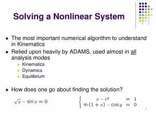
F i. R. r. H. h. F. Example: Linearization of a nonlinear model involving a nonlinear function of two variables.

E N D
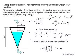
Fi R r H h F Example: Linearization of a nonlinear model involving a nonlinear function of two variables. The dynamic behavior of the liquid level h in the conical storage tank system shown in the figure can be shown to be represented below, where now the cross section area of the tank is given by: The tank model becomes where α and β are parameters defined by: Dr. Kalyana Veluvolu
This process model has two types of nonlinear functions: Fih-2 , a product of two functions, and h-3/2. We shall have to linearize each of these functions seperately around the steady state (hs, Fis). The linearization of f(h, Fi) = Fih-2 proceeds as follows: whereupon carrying out the indicated operations now gives: If we ignore the higher order terms. The steps involved in linearizing the second nonlinear term are no different from those illustrated in the previous example; the result is Dr. Kalyana Veluvolu
We may now introduce these expressions in place of corresponding nonlinear terms in Recalling that under steady-state conditions αFis=βhs1/2, and introducing the deviation variables y=(h-hs) and u = (Fi-Fis), the approximate linear model is obtained upon further simplification as: where the steady-state gain, and time constant associated with this approximate linear model, are given by: and Dr. Kalyana Veluvolu
If we desire an approximate transform-domain transfer function model, Laplace transformation again gives Note that the approximate linear model for the conical tank has the same process gain, K, as for the cylindirical tank; but the time constant is a much stronger function of the liquid level hs. Some important points to note about the results of these two illustrative examples are the following: • In each case, the approximate transfer function model is of the first-order process, with the time constants, and steady-state gain values dependent on the specific steady-state around which the system model was linearized. • Using such approximate transfer function models will give approximate results which are good in a small neighborhood around the initial steady-state; farther away from this steady-state the accuracy of the approximate results becomes poorer. • Using such approximate models, we are able to get a general (even if not 100% accurate) idea about the speed and magnitude of response to expect from any arbitrary nonlinear system. Numerical analysis can give more accurate information, but only about the specific input, starting from a specific operating condition for a specific set of parameters. Dr. Kalyana Veluvolu
Let us conclude with a comparison of the responses of the nonlinear model and an approximate linear model for the conical tank of the Example. Suppose that α=2, β=1, c=0.5 so that the nonlinear model is: while the approximate linear model has the transfer function which in the time domain is Dr. Kalyana Veluvolu
tank1.m tank.m clc;clear tss=4; [t,h]=ode45('tank1',0,tss,[0.5]); plot(t,h(:,1)) function hdot=tank1(t,h) hs=0.5; dfi=0.15; hdot=[1/(2*hs^2.5)*(hs-h+4*hs^0.5*dfi)]; Nonlinear model function hdot=tanknl1(t,h) alfa=2; beta=1; Fs=0.3536; dfi=0.05; Fi=Fs+dfi; hdot=[alfa*Fi/h^2-beta*h^(-1.5)]; clc;clear tss=4; [t,h]=ode45('tanknl1',0,tss,[0.5]); plot(t,h(:,1))
The step response for these models is shown in the Figure for steps of two different magnitudes. • For small magnitude step inputs, the linear model is a good approximation of the nonlinear model. • For large amplitude inputs the linear model predictions deviate somewhat from the nonlinear model behavior.
However, in some situations this may be inadequate (e.g. for the control of highly nonlinear processes) so the development of nonlinear controllers has featured prominently in process control in the last decade. Adaptive Control: A controller designed for the systems in the level control example in the previous example using the approximate transfer function model will function acceptably as long as the level, h, is maintaned at, or close to, the steady-state value hs. Under these conditions (h-hs) will be small enough to make the linear approximation adequate. However, if the level is required to change over a wide range, the farther away from hs the level gets, the poorer the linear approximation. Observe also from the approximate transfer function model that the apparent steady state-state gain and time constant are dependent on the steady-state around which the linearization was carried out. This implies that in going from one steady state to the other, the approximate process parameters will change. Dr. Kalyana Veluvolu
The main problem with applying the classical approach under these circumstances is that it ignores the fact that the characteristics of the approximate model must change as the process moves away from hs if the approximate model is to remain reasonably accurate. The immediate implication is that any controller designed on the basis of this changing approximate model must also have its parameters adjusted if it is to remain effective. In the adaptive control scheme, the controller parameters are adjusted (in an automatic fashion) to keep up with the changes in the process characteristics. We know intuitively that, if properly designed, this procedure will be a significant improvement over the classical scheme. There are various types of adaptive control methods, differing mainly in the way the controller parameters are adjusted. The three most popular methods are: scheduled adaptive control, model reference adaptive control, and self-tuning controllers. Dr. Kalyana Veluvolu
Parameter Adjustment Figure. Scheduled adaptive controller. Scheduled Adaptive Control A scheduled adaptive control method is one in which, as a result of a priori knowledge and easy quantification of what is responsible for the changes in the process charactersitics, the commensurate changes required in the controller parameters are programmed (or scheduled) ahead of time. This type of adaptive controller, sometimes referred to as gain scheduling, is illustrated by the block diagram in the following figure. Dr. Kalyana Veluvolu
Continuing with the example of liquid level system, the figure represents control of linearised approximation of the original nonlinear system. The approximation is in the sense that the process transfer function G(s) only holds good for a particular level of the liquid in the tank. If the level h changes drastically, the transfer function G(s) may fail to represent the original system even approximately. Then there is a need to change the transfer function G(s) to account for the change in level h. One way of doing this is through Scheduled adaptive controller shown in previous page. From the system transfer function it is seen that both K and τ are affected by the liquid level h. The effect on K is more prominent since it affects the system gain. The effect on the time constant is less apparent and not so prominent. Thus we only compansate for the effect of liquid level h on K. This is done in a way that the overall system gain KKc is constant. Notice that Dr. Kalyana Veluvolu
So, to keep KKc = K0 (a constant) This means that the controller gain Kc has to be adjusted inversely as the square root of the liquid level h. This is what will be done by the block represented as “Parameter adjustment” in the figure. More generally, if K = K(t), that is, the process gain changes with time, then to keep the product KKc constant it is necessary to adjust Kc inversely with respect to K(t), i.e. K(t) itself can be determined periodically by inserting a signal u into the process and monitoring the process output y. Dr. Kalyana Veluvolu
Table: Scheduled control of Valve Valve opening Kp Ti Td 0.0-0.15 1.7 95 23 0.15-0.22 2.0 89 22 0.22-0.35 2.9 82 21 0.35-1.0 4.4 68 17 In practice, it is often possible to find measured variables that correlate well with changes in process dynamics. These variables can be used to change the controller parameters, using a precalculated schedule. The controller parameters are computed off-line for several operating conditions and stored in memory. It is difficult to give general rules. Each case must be treated individually. The key question is to determine the auxiliary variables to be used as scheduling variables. It is necessary to have good insight into the dynamics of the process if gain scheduling is going to be used. The controller can be automatically tuned at a different operating points and the resulting tuning parameters can be saved and a schedule created. Example: The figure given below shows different valve characteristics, if the scheduling variable in a level control system is the opening of a control valve, then a schedule may look as in the Table: Flow Quick opening Linear Equal percentage Dr. Kalyana Veluvolu Position
Contol signal u Command signal uc Output y + PI f-1(c) f(u) G(s) - Nonlinear Valve Process Example: The nonlinearity of the valve is assumed to be: Let f-1 be an approximation of the inverse of the valve characteristics. To compensate for the nonlinearity, the output of the controller fed through this function before it is applied to the valve. This gives the relation: where c is the output of the PI controller Dr. Kalyana Veluvolu
15 10 0 2 Time 1 Figure. A crude approximation of valve characteristics. Assume that f(u)=u4 is approximated by two lines as shown in the figure. One from (0,0) to (1.3,3) and the other from (1.3,3) to (2,16). Then we have: Dr. Kalyana Veluvolu
Model Reference Adaptive Controller (MRAC) • The key component of the MRAC scheme is the reference model that consists of a reasonable closed-loop model of how the process should respond to a set-point change. This could be as simple as a reference trajectory, or it could be more detailed closed-loop model. The reference model output is compared with the actual process output and the observed error ᵋm is used to drive some adoptation scheme to cause the controller parameters to be adjusted so as to reduce ᵋm to zero. The adoptaion scheme could be some control parameter optimization algorithm that reduces the integral squared value of ᵋm or some other procedure. This is an adaptive control technique where the performance specifications are given in terms of a model. The model represents the ideal response of the process to a command signal. The controller has two loops: • The inner loop, which is an ordinary feedback loop consisting of the process and the controller. • The outer loop, which adjust the controller parameters in such a way that the error e = y- ym is small (not trivial) Dr. Kalyana Veluvolu
Tracking error: Introduce the cost function J: Where θ is a vector of controller parameters. Change the parameters in the direction of the negative gradient of e2.
is called the sensitivity derivative. It indicates how the error is influenced by the adjustable parameters θ. MIT Rule Example: Process: Model: Controller: Closed loop system:
Ideal controller parameters for perfect model-following Derivation of adaptive law Error: where Sensitivity derivatives
Approximate where
MRAC of Pendulum d2 d1 dc T • System Keith Sevcik
MRAC of Pendulum Model ymodel Adjustment Mechanism Controller Parameters uc Controller u yplant • Controller will take form: Keith Sevcik
MRAC of Pendulum • Following process as before, write equation for error, cost function, and update rule: sensitivity derivative Keith Sevcik
MRAC of Pendulum • Assuming controller takes the form:
MRAC of Pendulum • If reference model is close to plant, can approximate:
MRAC of Pendulum • From MIT rule, update rules are then:
MRAC of Pendulum Reference Model ymodel - + Π + - uc yplant θ1 e Plant Π θ2 Π Π • Block Diagram Keith Sevcik
MRAC of Pendulum • Simulation block diagram (NOTE: Modeled to reflect control of DC motor) Keith Sevcik
Simulation with small gamma = UNSTABLE! Keith Sevcik
MRAC of Pendulum • Solution: Add PD feedback Keith Sevcik
MRAC of Pendulum • Simulation results with varying gammas Keith Sevcik