Download
1 / 46
460 likes | 675 Views
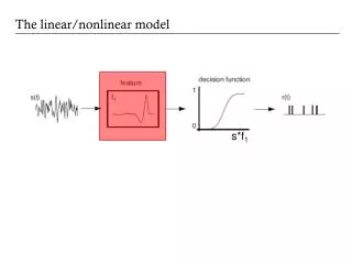
The linear/nonlinear model. s*f 1. Th e spike-triggered average. Dimensionality reduction. More generally, one can conceive of the action of the neuron or neural system as s electing a low dimensional subset of its inputs. Start with a very high dimensional description

E N D
Dimensionality reduction More generally, one can conceive of the action of the neuron or neural system as selecting a low dimensional subset of its inputs. Start with a very high dimensional description (eg. an image or a time-varying waveform) and pick out a small set of relevant dimensions. P(response | stimulus) P(response | s1, s2, .., sn) s2 s3 s(t) s1 s3 sn s4 s5 s.. s.. s.. s2 s1 S(t) = (S1,S2,S3,…,Sn)
Linear filtering Linear filtering = convolution = projection s2 s3 s1 Stimulus feature is a vector in a high-dimensional stimulus space
Determining the nonlinear input/output function The input/output function is: which can be derived from data using Bayes’ rule:
Nonlinear input/output function Tuning curve: P(spike|s) = P(s|spike) P(spike) / P(s) Tuning curve: P(spike|s) = P(s|spike) P(spike) / P(s) P(s) P(s|spike) P(s) P(s|spike) s s
Models with multiple features Linear filters & nonlinearity: r(t) = g(f1*s, f2*s, …, fn*s)
covariance Determining linear features from white noise Gaussian prior stimulus distribution Spike-conditional distribution Spike-triggered average
Identifying multiple features The covariance matrix is Stimulus prior Spike-triggered stimulus correlation Spike-triggered average • Properties: • The number of eigenvalues significantly different from zero • is the number of relevant stimulus features • The corresponding eigenvectors are the relevant features • (or span the relevant subspace) Bialek et al., 1988; Brenner et al., 2000; Bialek and de Ruyter, 2005
Inner and outer products uv = Sui vi uv = projection of u onto v uu = length of u uxv = M where Mij = uivj
Eigenvalues and eigenvectors M u=lu
Singular value decomposition n m = M U x S x V
Principal component analysis M M* = (U S V)(V*S*U*) =U S (V V*) S*U* = U S S*U* C= ULU*
Identifying multiple features The covariance matrix is Stimulus prior Spike-triggered stimulus correlation Spike-triggered average • Properties: • The number of eigenvalues significantly different from zero • is the number of relevant stimulus features • The corresponding eigenvectors are the relevant features • (or span the relevant subspace) Bialek et al., 1988; Brenner et al., 2000; Bialek and de Ruyter, 2005
A toy example: a filter-and-fire model Let’s develop some intuition for how this works: a filter-and-fire threshold-crossing model with AHP Keat, Reinagel, Reid and Meister, Predicting every spike. Neuron (2001) • Spiking is controlled by a single filter, f(t) • Spikes happen generally on an upward threshold crossing of • the filtered stimulus • expect 2 relevant features, the filter f(t) and its time derivative f’(t)
STA f(t) f'(t) Covariance analysis of a filter-and-fire model
Some real data Example: rat somatosensory (barrel) cortex Ras Petersen and Mathew Diamond, SISSA Record from single units in barrel cortex
Normalisedvelocity Pre-spike time (ms) White noise analysis in barrel cortex Spike-triggered average:
White noise analysis in barrel cortex Is the neuron simply not very responsive to a white noise stimulus?
Covariance matrices from barrel cortical neurons Prior Spike- triggered Difference
0.4 0.3 0.2 0.1 Velocity 0 -0.1 -0.2 -0.3 -0.4 150 100 50 0 Pre-spike time (ms) Eigenspectrum from barrel cortical neurons Eigenspectrum Leading modes
Input/output relations from barrel cortical neurons Input/output relations wrt first two filters, alone: and in quadrature:
0.4 0.3 0.2 Velocity (arbitrary units) 0.1 0 -0.1 -0.2 -0.3 150 100 50 0 Pre-spike time (ms) Less significant eigenmodes from barrel cortical neurons How about the other modes? Next pair with +veeigenvalues Pair with -veeigenvalues
Negative eigenmode pair Input/output relations for negative pair Firing rate decreases with increasing projection: suppressive modes
Salamander retinal ganglion cells perform a variety of computations Michael Berry
Complex cells in V1 Rust et al., Neuron 2005
Basic types of computation • integrators • H1, some single cortical neurons • differentiators • Retina, simple cells, HH neuron, auditory neurons • frequency-power detectors • V1 complex cells, somatosensory, auditory, retina
When have you done a good job? • When the tuning curve over your variable is interesting. • How to quantify interesting?
When have you done a good job? Tuning curve: P(spike|s) = P(s|spike) P(spike) / P(s) Tuning curve: P(spike|s) = P(s|spike) P(spike) / P(s) Boring: spikes unrelated to stimulus Interesting: spikes are selective P(s) P(s|spike) P(s) P(s|spike) s s Goodness measure: DKL(P(s|spike) | P(s))
Maximally informative dimensions Sharpee, Rust and Bialek, Neural Computation, 2004 Choose filter in order to maximize DKL between spike-conditional and prior distributions Equivalent to maximizing mutual information between stimulus and spike P(s) P(s|spike) Does not depend on white noise inputs Likely to be most appropriate for deriving models from natural stimuli s = I*f
Finding relevant features • Single, best filter determined by the first moment • A family of filters derived using the second moment • Use the entire distribution: information theoretic methods Removes requirement for Gaussian stimuli
Less basic coding models Linear filters & nonlinearity: r(t) = g(f1*s, f2*s, …, fn*s) …shortcomings?
Less basic coding models GLM: r(t) = g(f1*s + f2*r) Pillow et al., Nature 2008; Truccolo, .., Brown, J. Neurophysiol. 2005
Less basic coding models GLM: r(t) = g(f*s +h*r) …shortcomings?
Less basic coding models GLM: r(t) = g(f1*s + h1*r1 + h2*r2 +…) …shortcomings?
Poisson spiking Shadlen and Newsome, 1998
Poisson spiking Properties: Distribution: PT[k] = (rT)kexp(-rT)/k! Mean: <x> =rT Variance: Var(x)=rT Fano factor: F = 1 Interval distribution: P(T) = r exp(-rT)
Poisson spiking in the brain Area MT A B Data fit to: variance = A meanB Fano factor
Poisson spiking in the brain How good is the Poisson model? ISI analysis ISI distribution generated from a Poisson model with a Gaussian refractory period ISI Distribution from an area MT Neuron