Download
1 / 29
290 likes | 425 Views
NCAR. ATEC. USWRP. FAA. Object-based Evaluation of Weather Forecasts: Application to NWP models. Chris Davis (ESSL/MMM and RAL) Collaborators: Barb Brown (RAL), Daran Rife (RAL) and Randy Bullock (RAL). Objects? Events (time series) Features (temporal or spatial)

E N D
NCAR ATEC USWRP FAA Object-based Evaluation of Weather Forecasts: Application to NWP models Chris Davis (ESSL/MMM and RAL) Collaborators: Barb Brown (RAL), Daran Rife (RAL) and Randy Bullock (RAL) Objects? • Events (time series) • Features (temporal or spatial) • Anomalies (time or space)
Why Objects? • Dimension reduction ~ 107-109 variables per simulation reduced to ~ 102 variables • Objects directly related to phenomena • Localized (discrete, non-linear) • Episodic (non-periodic) • Used for deterministic, probabilistic and stochastic forecasts. • Relevant to users
O F O F F O Match Obs YY YN F O O F Fcst NY NN Traditional “Measures”-Based Approach Consider forecasts and observations of some dichotomous field on a grid: CSI = 0 for first 4; CSI > 0 for the 5th Critical Success Index CSI=YY/(YY+NY+YN) Equitable Threat Score ETS=(YY-e)/(YY+NY+YN-e), where e=success due to chance Non-diagnostic and utra-sensitive to small errors in simulation of localized phenomena!
Object Distributions Object Matching • Decide whether forecast object has observed counterpart • Evaluate errors in attributes of matched objects • Keep track of unmatched objects • Analyze statistics of objects in forecasts and observations • Apply to series of forecasts or climate simulations
Objects in One Dimension MM5, Dx=3.3 km, WSMR Time Series of east-west 10-m wind component
Diurnal Timing of Wind Changes • Compute all objects from forecasts and observations separately at each point (changes exceeding ±s from respective distributions. • Compute the mode of occurrence time (i.e., hour of the day). • Plot spatial distribution of time for positive and negative changes (u-component). • Plot analogous times from observations (discrete points)
Diurnal Timing of Wind Changes Zonal Wind Zonal Wind time time Sunset Sunrise
Max skill based on perturbed obs with sobs =1.5 m/s Match Obs YY YN Fcst NY NN Comparison of Fine and Coarse-resolution Models Equitable Threat Score for positive objects (2-h changes of wind > +s) YY=Forecast and observed object of the same sign occur with the same 12-h forecast period. High-resolution forecasts better, but not by much! ETS=(YY-e)/(YY+NY+YN-e), where e=success due to chance
Defining Rain Areas (2-D) f(x,y) Restore original field where h(x,y) =1
Alternative Object Definitions • Cluster Analysis • Wavelet Decomposition • Spectral Decomposition • Planetary waves • Diurnal cycle of temperature • Asymmetries on vortices y y 8 clusters in (x,y,precip) space x Marzban and Sandgathe (WGNE Verif. Workshop, 2004)
f o Object Distributions Object Matching • Matching a function of separation distance only (‘x’ or ‘t’); more general approaches being examined (B. Brown seminar) • Acceptable separation proportional to object size 22-km EH July-Aug. 2001
Verification of 4-km WRF • WRF (ARW core) on 500x500x34 grid • 00 UTC initialization from 00 UTC Eta • Only 13-36 h hourly precipitation accumulations • Stage IV interpolated to WRF grid • May 3 - July 14, 2003 • Subjective verification in Done et al. (2004, ASL)
L W Object Attributes • Intensity (percentile value) • Area (# grid points > T) • Centroid • Axis angle (rel. to E-W) • Aspect ratio (W/L) • Fractional Area • Curvature 75th Percentile Median 25th Percentile R=16 km; T = 5 mm h-1 Raw Forecast (28 h, 04 UTC 11 June)
Scaling of Rain Areas + = WRF; o = Obs L W
Distribution of Spatial Errors yf-yo xf-xo
Matching and Forecast “Skill” Much greater dependence of forecast error on the size of objects than on forecast lead time Match Obs YY YN Fcst NY CSI=YY/(YY+NY+YN)
Time Lat Lon Objects in Three Dimensions (x,y,t)
Time Lat Lon
Constructing 3-D Objects • Match rain areas separated by dt within a given data set. • Choose maximum separation so that c1 < D/dt < c2 • Treat matched pair as new object with duration 2dt. • Match all objects with duration 2dt (get objects of duration 3dt). • Repeat Schematic in 2-D (x,y) space Time
Matching 3-D “Rain Systems” • Centroid separation < 4W (W=width) • Time centroid separation < 3 h • Longevity within factor of 2 • Minimum 3-h duration for model systems • 75th percentile rainfall above average Match Obs L YY YN Fcst W NY CSI=YY/(YY+NY+YN)
Biases for 3-D Objects CSI Late Systems last too long
Biases for 3-D Objects Systems too large Small high bias on heavier rain
“Resolution” Dependence 22-km Cu Param Lighter Rain Heavier Rain 4-km No Cu Param
Comparison with Subjective Verification • Done et al. (2004, ASL) conducted a subjective verification of MCSs using the same data. Comparison? • This study • Minimum allowed separation = 4W (average W ~ 80 km) • 3-h duration of fcst systems • Relatively automated • Done et al. • Minimum separation = 3º latitude (333 km) • required 6 h duration of both fcst and obs MCSs • Exhausted and nearly blinded the investigators This study Average CSI: 0.5 CSI for systems with T≥6 h: 0.38 Done et al. CSI for separation < 333 km: 0.32
Extensions • Probabilistic Forecasts • Climate Simulations • Extreme Events
Findings (Terrain Flows) • Winds near complex terrain only marginally more predictable with higher resolution • Repeatable diurnal circulations small contributors of variance (Rife et al. 2004, MWR) • Larger-scale terrain features exert broad influence • Best application of high-resolution is stochastic, not deterministic • Regional climate simulations • Ensemble spread
Findings (Rainfall) • Scaling laws for rainfall objects (vs. object size) • Exponential decay of frequency • Elongation and SW-NE orientation (frontal?) • Decrease of fractional area • Diurnal cycle of errors (size, intensity, timing) • Systems last too long (nocturnal) • Systems too large (daytime) • Positive bias for heavier rainfall • Parameterized convection inhibits correct rainfall distribution • Favorable comparison with subjective verification (relation to Weisman 1-2-3 verification system still unknown)