Modeling & Analysis

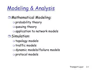
1. Modeling & Analysis • Mathematical Modeling: • probability theory • queuing theory • application to network models • Simulation: • topology models • traffic models • dynamic models/failure models • protocol models Transport Layer

2. Simulation tools • VINT (Virtual InterNet Testbed): • catarina.usc.edu/vint [USC/ISI, UCB,LBL,Xerox] • network simulator (NS), network animator (NAM) • library of protocols: • TCP variants • multicast/unicast routing • routing in ad-hoc networks • real-time protocols (RTP) • …. Other channel/protocol models & test-suites • extensible framework (Tcl/tk & C++) • Check the ‘Simulator’ link thru the class website Transport Layer

3. OPNET: • commercial simulator • strength in wireless channel modeling • GlomoSim (QualNet): UCLA, parsec simulator • Research resources: • ACM & IEEE journals and conferences • SIGCOMM, INFOCOM, Transactions on Networking (TON), MobiCom • IEEE Computer, Spectrum, ACM Communications magazine • www.acm.org, www.ieee.org Transport Layer

4. Modeling using queuing theory • Let: • N be the number of sources • M be the capacity of the multiplexed channel • R be the source data rate •  be the mean fraction of time each source is active, where 0<1 Transport Layer

5. Transport Layer

6. if N.R=M then input capacity = capacity of multiplexed link => TDM • if N.R>M but .N.R<M then this may be modeled by a queuing system to analyze its performance Transport Layer

7. Queuing system for single server Transport Layer

8.  is the arrival rate • Tw is the waiting time • The number of waiting items w=.Tw • Ts is the service time •  is the utilization ‘fraction of the time the server is busy’, =.Ts • The queuing time Tq=Tw+Ts • The number of queued items (i.e. the queue occupancy) q=w+=.Tq Transport Layer

9. =.N.R, Ts=1/M • =.Ts=.N.R.Ts=.N.R/M • Assume: - random arrival process (Poisson arrival process) • constant service time (packet lengths are constant) • no drops (the buffer is large enough to hold all traffic, basically infinite) • no priorities, FIFO queue Transport Layer

10. Inputs/Outputs of Queuing Theory • Given: • arrival rate • service time • queuing discipline • Output: • wait time, and queuing delay • waiting items, and queued items Transport Layer

11. Queue Naming: X/Y/Z • where X is the distribution of arrivals, Y is the distribution of the service time, Z is the number of servers • G: general distribution • M: negative exponential distribution • (random arrival, poisson process, exponential inter-arrival time) • D: deterministic arrivals (or fixed service time) Transport Layer

12. Transport Layer

13. M/D/1: • Tq=Ts(2-)/[2.(1-)], • q=.Tq=+2/[2.(1-)] Transport Layer

14. Transport Layer

15. Transport Layer

16. Transport Layer

17. As  increases, so do buffer requirements and delay • The buffer size ‘q’ only depends on  Transport Layer

18. Queuing Example • If N=10, R=100, =0.4, M=500 • Or N=100, M=5000 • =.N.R/M=0.8, q=2.4 • a smaller amount of buffer space per source is needed to handle larger number of sources • variance of q increases with  • For a finite buffer: probability of loss increases with utilization >0.8 undesirable Transport Layer

19. Chapter 3Transport Layer Computer Networking: A Top Down Approach 4th edition. Jim Kurose, Keith RossAddison-Wesley, July 2007. Transport Layer

20. Transport Layer

21. Transport Layer

22. rdt_send():called from above, (e.g., by app.). Passed data to deliver to receiver upper layer deliver_data():called by rdt to deliver data to upper udt_send():called by rdt, to transfer packet over unreliable channel to receiver rdt_rcv():called when packet arrives on rcv-side of channel Reliable data transfer: getting started send side receive side Transport Layer

23. Flow Control • End-to-end flow and Congestion control study is complicated by: • Heterogeneous resources (links, switches, applications) • Different delays due to network dynamics • Effects of background traffic • We start with a simple case: hop-by-hop flow control Transport Layer

24. Hop-by-hop flow control • Approaches/techniques for hop-by-hop flow control • Stop-and-wait • sliding window • Go back N • Selective reject Transport Layer

25. underlying channel perfectly reliable no bit errors, no loss of packets stop and wait Stop-and-wait: reliable transfer over a reliable channel Sender sends one packet, then waits for receiver response Transport Layer

26. underlying channel may flip bits in packet checksum to detect bit errors the question: how to recover from errors: acknowledgements (ACKs): receiver explicitly tells sender that pkt received OK negative acknowledgements (NAKs): receiver explicitly tells sender that pkt had errors sender retransmits pkt on receipt of NAK new mechanisms for: error detection receiver feedback: control msgs (ACK,NAK) rcvr->sender channel with bit errors Transport Layer

27. Stop-and-wait operation Summary • Stop and wait: • sender awaits for ACK to send another frame • sender uses a timer to re-transmit if no ACKs • if ACK is lost: • A sends frame, B’s ACK gets lost • A times out & re-transmits the frame, B receives duplicates • Sequence numbers are added (frame0,1 ACK0,1) • timeout: should be related to round trip time estimates • if too small  unnecessary re-transmission • if too large  long delays Transport Layer

28. Stop-and-wait with lost packet/frame Transport Layer

29. Transport Layer

30. Transport Layer

31. Stop and wait performance • utilization – fraction of time sender busy sending • ideal case (error free) • u=Tframe/(Tframe+2Tprop)=1/(1+2a), a=Tprop/Tframe Transport Layer

32. example: 1 Gbps link, 15 ms e-e prop. delay, 1KB packet: Performance of stop-and-wait L (packet length in bits) 8kb/pkt T = = = 8 microsec transmit R (transmission rate, bps) 10**9 b/sec • U sender: utilization – fraction of time sender busy sending • 1KB pkt every 30 msec -> 33kB/sec thruput over 1 Gbps link • network protocol limits use of physical resources! Transport Layer

33. stop-and-wait operation sender receiver first packet bit transmitted, t = 0 last packet bit transmitted, t = L / R first packet bit arrives RTT last packet bit arrives, send ACK ACK arrives, send next packet, t = RTT + L / R Transport Layer

34. Sliding window techniques • TCP is a variant of sliding window • Includes Go back N (GBN) and selective repeat/reject • Allows for outstanding packets without Ack • More complex than stop and wait • Need to buffer un-Ack’ed packets & more book-keeping than stop-and-wait Transport Layer

35. Pipelining: sender allows multiple, “in-flight”, yet-to-be-acknowledged pkts range of sequence numbers must be increased buffering at sender and/or receiver Two generic forms of pipelined protocols: go-Back-N, selective repeat Pipelined (sliding window) protocols Transport Layer

36. Pipelining: increased utilization sender receiver first packet bit transmitted, t = 0 last bit transmitted, t = L / R first packet bit arrives RTT last packet bit arrives, send ACK last bit of 2nd packet arrives, send ACK last bit of 3rd packet arrives, send ACK ACK arrives, send next packet, t = RTT + L / R Increase utilization by a factor of 3! Transport Layer

37. Sender: k-bit seq # in pkt header “window” of up to N, consecutive unack’ed pkts allowed Go-Back-N • ACK(n): ACKs all pkts up to, including seq # n - “cumulative ACK” • may receive duplicate ACKs (more later…) • timer for each in-flight pkt • timeout(n): retransmit pkt n and all higher seq # pkts in window Transport Layer

38. ACK-only: always send ACK for correctly-received pkt with highest in-order seq # may generate duplicate ACKs need only remember expected seq num out-of-order pkt: discard (don’t buffer) -> no receiver buffering! Re-ACK pkt with highest in-order seq # GBN: receiver side Transport Layer

39. GBN inaction Transport Layer

40. receiver individually acknowledges all correctly received pkts buffers pkts, as needed, for eventual in-order delivery to upper layer sender only resends pkts for which ACK not received sender timer for each unACKed pkt sender window N consecutive seq #’s limits seq #s of sent, unACKed pkts Selective Repeat Transport Layer

41. Selective repeat: sender, receiver windows Transport Layer

42. Selective repeat in action Transport Layer

43. performance: • selective repeat: • error-free case: • if the window is w such that the pipe is fullU=100% • otherwise U=w*Ustop-and-wait=w/(1+2a) • in case of error: • if w fills the pipe U=1-p • otherwise U=w*Ustop-and-wait=w(1-p)/(1+2a) Transport Layer

44. full duplex data: bi-directional data flow in same connection MSS: maximum segment size connection-oriented: handshaking (exchange of control msgs) init’s sender, receiver state before data exchange flow controlled: sender will not overwhelm receiver point-to-point: one sender, one receiver reliable, in-order byte stream: no “message boundaries” pipelined: TCP congestion and flow control set window size send & receive buffers TCP: OverviewRFCs: 793, 1122, 1323, 2018, 2581 Transport Layer

45. 32 bits source port # dest port # sequence number acknowledgement number head len not used Receive window U A P R S F checksum Urg data pnter Options (variable length) application data (variable length) TCP segment structure URG: urgent data (generally not used) counting by bytes of data (not segments!) ACK: ACK # valid PSH: push data now (generally not used) # bytes rcvr willing to accept RST, SYN, FIN: connection estab (setup, teardown commands) Internet checksum (as in UDP) Transport Layer

46. Receive window: credit (in octets) that the receiver is willing to accept from the sender starting from ack # • flags: • SYN: synchronizing at initail connection time • FIN: end of sender data • PSH: when used at sender the data is transmitted immediately, when at receiver, it is accepted immediately • options: • window scale factor (WSF): actual window = 2Fxwindow field, where F is the number in the WSF • timestamp option: helps in RTT (round-trip-time) calculations Transport Layer

47. credit allocation scheme • (A=i,W=j) [A=Ack, W=window]: receiver acks up to ‘i-1’ bytes and allows/anticipates i up to i+j-1 • receiver can use the cumulative ack option and not respond immediately • performance: depends on • transmission rate, propagation, window size, queuing delays, retransmission strategy which depends on RTT estimates that affect timeouts and are affected by network dynamics, receive policy (ack), background traffic….. it is complex! Transport Layer

48. Seq. #’s: byte stream “number” of first byte in segment’s data ACKs: seq # of next byte expected from other side cumulative ACK Q: how receiver handles out-of-order segments A: TCP spec doesn’t say, - up to implementor time TCP seq. #’s and ACKs Host B Host A User types ‘C’ Seq=42, ACK=79, data = ‘C’ host ACKs receipt of ‘C’, echoes back ‘C’ Seq=79, ACK=43, data = ‘C’ host ACKs receipt of echoed ‘C’ Seq=43, ACK=80 simple telnet scenario Transport Layer

49. TCP retransmission strategy: • TCP performs end-to-end flow/congestion control and error recovery • TCP depends on implicit congestion signaling and uses an adaptive re-transmission timer, based on average observation of the ack delays. Transport Layer

50. Ack delays may be misleading due to the following reasons: • Cumulative acks render this estimate inaccurate • Abrupt changes in the network • If ack is received for a re-transmitted packet, sender cannot distinguish between ack for the original packet and ack for the re-transmitted packet Transport Layer