Download
1 / 41
410 likes | 487 Views
Visual FAQ’s on Real Options Celebrating the Fifth Anniversary of the Website: Real Options Approach to Petroleum Investments http://www.puc-rio.br/marco.ind/. Real Options 2000 Conference Capitalizing on Uncertainty and Volatility in the New Millennium September 25, 2000 - Chicago.

E N D
Visual FAQ’s on Real OptionsCelebrating the Fifth Anniversary of the Website:Real Options Approach to Petroleum Investmentshttp://www.puc-rio.br/marco.ind/ Real Options 2000 ConferenceCapitalizing on Uncertainty and Volatility in the New MillenniumSeptember 25, 2000 - Chicago By: Marco Antônio Guimarães Dias Petrobras and PUC-Rio, Brazil
Visual FAQ’s on Real Options • Selection of frequently asked questions (FAQ’s) by practitioners and academics • Something comprehensive but I confess some bias in petroleum questions • Use of some facilities to visual answer • Real options models present two results: • The value of the investment oportunity (option value) • How much to pay (or sell) for an asset with options? • The decision rule (thresholds) • Invest now? Wait and See? Abandon? Expand the production? Switch use of an asset? • Option value and thresholds are the focus of most visual FAQ’s
Visual FAQ’s on Real Options: 1 • Are the real options premium important? Real Option Premium = Real Option Value - NPV • Answer with an analogy: • Investments can be viewed as call options • You get an operating project V (like a stock) by paying the investment cost I (exercise price) • Sometimes this option has a time of expiration (petroleum, patents, etc.), sometimes is perpetual (real estate, etc.) • Suppose a 3 years to expiration petroleum undeveloped reserve. The immediate exercise of the option gets the NPV NPV = V - I
Real Options Premium • The options premium can be important or not, depending of the of the project moneyness
Visual FAQ’s on Real Options: 2 • What are the effects of interest rate, volatility, and other parameters in both option value and the decision rule? • Answer with “Timing Suite” • Three spreadsheets that uses a simple model analogy of real options problem with American call option • Lets go to the Excel spreadsheets to see the effects
Visual FAQ’s on Real Options: 3 • Where the real options value comes from? • Why real options value is different of the static net present value (NPV)? • Answer with example: option to expand • Suppose a manager embed an option to expand into her project, by a cost of US$ 1 million • The static NPV = - 5 million if the option is exercise today, and in future is expected the same negative NPV • Spending a million $ for an expected negative NPV: Is the manager becoming crazy?
Uncertainty Over the Expansion Value • Considering combined uncertainties: in product prices and demand, exercise price of the real option, operational costs, etc., the future value (2 years ahead) of the expansion has an expected value of $ - 5 million • The traditional discount cash will not recommend to embed an option to expansion which is expected to be negative • But the expansion is an option, not an obligation!
Option to Expand the Production • Rational managers will not exercise the option to expand @ t = 2 years in case of bad news (negative value) • Option will be exercised only if the NPV > 0. So, the unfavorable scenarios will be pruned (for NPV < 0, value = 0) • Options asymmetry leverage prospect valuation. Option = + 5
Real Options Asymmetry and Valuation • The visual equation for “Where the options value comes from?” + = Prospect Valuation Traditional Value = - 5 Options Value(T) = + 5
E&P Process and Options Oil/Gas Success Probability = p • Drill the wildcat? Wait? Extend? • Revelation, option-game: waiting incentives Expected Volume of Reserves = B Revised Volume = B’ • Appraisal phase: delineation of reserves • Technical uncertainty: sequential options • Delineated but Undeveloped Reserves. • Develop? “Wait and See” for better conditions? Extend the option? • Developed Reserves. • Expand the production? • Stop Temporally? Abandon?
Option to Expand the Production • Analyzing a large ultra-deepwater project in Campos Basin, Brazil, we faced two problems: • Remaining technical uncertainty of reservoirs is still important. In this specific case, the better way to solve the uncertainty is by looking the production profile instead drilling additional appraisal wells • In the preliminary development plan, some wells presented both reservoir risk and small NPV. • Some wells with small positive NPV (not “deep-in-the-money”) and others even with negative NPV • Depending of the initial production information, some wells can be not necessary • Solution: leave these wells as optional wells • Small investment to permit a fast and low cost future integration of these wells, depending of both market (oil prices, costs) and the production profile response
Modeling the Option to Expand • Define the quantity of wells “deep-in-the-money” to start the basic investment in development • Define the maximum number of optional wells • Define the timing (or the accumulated production) that the reservoir information will be revealed • Define the scenarios (or distributions) of marginal production of each optional well as function of time. • Consider the depletion if we wait after learn about reservoir • Add market uncertainty (reversion + jumps for oil prices) • Combine uncertainties using Monte Carlo simulation (risk-neutral simulation if possible, next FAQ) • Use optimization method to consider the earlier exercise of the option to drill the wells, and calculate option value • Monte Carlo for American options is a frontier research area • Petrobras-PUC project: Monte Carlo for American options
Visual FAQ’s on Real Options: 4 • Does risk-neutral valuation mean that investors are risk-neutral? • What is the difference between real simulation and risk-neutral simulation? • Answers • Risk-neutral valuation (RNV) does not assume investors or firms with risk-neutral preferences • RNV does not use real probabilities. It uses risk neutral probabilities (“martingale measure”) • Real simulation: real probabilities, uses real drift a • Risk-neutral simulation: the sample paths are risk-adjusted. It uses a risk-neutral drift: a’ = r - d
Geometric Brownian Motion Simulation Pt = P0 exp{ (a - 0.5 s2) Dt + s N(0, 1) } Pt = P0 exp{ (r - d - 0.5 s2) Dt + s N(0, 1) } • The real simulation of a GBM uses the real drift a. The price at future time t is given by: • By sampling the standard Normal distribution N(0, 1) you get the values forPt • With real drift use a risk-adjusted (to P) discount rate • The risk-neutral simulation of a GBM uses the risk-neutral drift a’ = r - d. Theprice at t is: • With risk-neutral drift, the correct discount rate is the risk-free interest rate.
Risk-Neutral Simulation x Real Simulation • For the underlying asset, you get the same value: • Simulating with real drift and discounting with risk-adjusted discount rate r ( where r = a + d ) • Or simulating with risk-neutral drift (r - d) but discounting with the risk-free interest rate (r) • For an option/derivative, the same is not true: • Risk-neutral simulation gives the correct option result (discounting with r) but the real simulation does not gives the correct value (discounting with r) • Why? Because the risk-adjusted discount rate is “adjusted” to the underlying asset, not to the option • Risk-neutral valuation is based on the absence of arbitrage, portfolio replication (complete market) • Incomplete markets: see next FAQ
Visual FAQ’s on Real Options: 5 • Is possible to use real options for incomplete markets? • What change? What are the possible ways? • Answer: Yes, is possible to use. • For incomplete markets the risk-neutral probability (martingale measure) is not unique • So, risk-neutral valuation is not rigorously correct because there is a lack of market values • Academics and practitioners use some ways to estimate the real option value, see next slide
Incomplete Markets and Real Options • In case of incomplete market, the alternatives to real options valuation are: • Assume that the market is approximately complete (your estimative of market value is reliable) and use risk-neutral valuation (with risk-neutral probability) • Assume firms are risk-neutral and discount with risk-free interest rate (with real probability) • Specify preferences (the utility function) of single-agent or the equilibrium at detailed level (Duffie) • Used by finance academics. In practice is difficult to specify the utility of a corporation (managers, stockholders) • Use the dynamic programming framework with an exogenous discount rate • Used by academics economists: Dixit & Pindyck, Lucas, etc. • Corporate discount rate express the corporate preferences?
Visual FAQ’s on Real Options: 6 • Is true that mean-reversion always reduces the options premium? • What is the effect of jumps in the options premium? • Answers: • First, we’ll see some different processes to model the uncertainty over the oil prices (for example) • Second, we’ll compare the option premium for an oilfield using different stochastic processes • All cases are at-the-money real options (current NPV = 0) • The equilibrium price is 20 $/bbl for all reversion cases
Geometric Brownian Motion (GBM) • This is the most popular stochastic process, underlying the famous Black-Scholes-Merton options equation • GBM: expected curve is a exponential growth (or decrease); prices have a log-normal distribution in every future time; and the variance grows linearly with the time
Mean-Reverting Process • In this process, the price tends to revert toward a long-run average price (or an equilibrium level) P. • Model analogy: spring (reversion force is proportional to the distance between current position and the equilibrium level). • In this case, variance initially grows and stabilize afterwards • Charts: the variance of distributions stabilizes after ti
Nominal Prices for Brent and Similar Oils (1970-1999) Jumps-down Jumps-up • We see oil prices jumps in both directions, depending of the kind of abnormal news: jumps-up in 1973/4, 1978/9, 1990, 1999; and jumps-down in 1986, 1991, 1997
Mean-Reversion + Jumps for Oil Prices where: • Adopted in the Marlim Project Finance (equity modeling) a mean-reverting process with jumps: (the probability of jumps) • The jump size/direction are random: f ~ 2N • In case of jump-up, prices are expected to double • OBS: E(f)up = ln2 = 0.6931 • In case of jump-down, prices are expected to halve • OBS: ln(½) = - ln2 = - 0.6931 (jump size)
Equation for Mean-Reversion + Jumps discrete process (jumps) continuous (diffusion) process variation of the stochastic variable for time interval dt uncertainty over the continuous process (reversion) { { mean-reversion drift: positive drift if P < P negative drift if P > P uncertainty over the discrete process (jumps) • The interpretation of the jump-reversion equation is:
Mean-Reversion x GBM: Option Premium • The chart compares mean-reversion with GBM for an at-the-money project at current 25 $/bbl • NPV is expected to revert from zero to a negative value Reversion in all cases: to 20 $/bbl
Mean-Reversion with Jumps x GBM • Chart comparing mean-reversion with jumps versus GBM for an at-the-money project at current 25 $/bbl • NPV still is expected to revert from zero to a negative value
Mean-Reversion x GBM • Chart comparing mean-reversion with GBM for an at-the-money project at current 15 $/bbl (suppose) • NPV is expected to revert from zero to a positive value
Mean-Reversion with Jumps x GBM • Chart comparing mean-reversion with jumps versus GBM for an at-the-money project at current 15 $/bbl (suppose) • Again NPV is expected to revert from zero to a positive value
Visual FAQ’s on Real Options: 7 • How to model the effect of the competitor entry in my investment decisions? • Answer : option-games, the combination of the real options with game-theory • First example: Duopoly under Uncertainty (Dixit & Pindyck, 1994; Smets, 1993) • Demand for a product follows a GBM • Only two players in the market for that product (duopoly)
Duopoly Entry under Uncertainty • The leader entry threshold: both players are indifferent about to be the leader or the follower. • Entry: NPV > 0 but earlier than monopolistic case
Other Example: Oil Drilling Game Company Y tract Company X tract • Oil exploration: the waiting game of drilling • Two companies X and Y with neighbor tracts and correlated oil prospects: drilling reveal information • If Y drills and the oilfield is discovered, the success probability for X’s prospect increases dramatically. If Y drilling gets a dry hole, this information is also valuable for X. • Here the effect of the competitor presence is the opposite: to increase the value of waiting to invest
Visual FAQ’s on Real Options: 8 • Does Real Options Theory (ROT) speed up the firms investments or slow down investments? • Answer: depends of the kind of investment • ROT speeds up today strategic investments that create options to invest in the future. Examples: investment in capabilities, training, R&D, exploration, new markets... • ROT slows down large irreversible investment of projects with positive NPV but not “deep in the money” • Large projects but with high profitability (“deep in the money”) must be done by both ROT and static NPV.
Visual FAQ’s on Real Options: 9 • Is possible real options theory to recommend investment in a negative NPV project? • Answer: yes, mainly sequential options with investment revealing new informations • Example: exploratory oil prospect (Dias 1997) • Suppose a “now or never” option to drill a wildcat • Static NPV is negative and traditional theory recommends to give up the rights on the tract • Real options will recommend to start the sequential investment, and depending of the information revealed, go ahead (exercise more options) or stop
Sequential Options (Dias, 1997) “Compact Decision-Tree” • Traditional method, looking only expected values, undervaluate the prospect (EMV = - 5 MM US$): • There are sequential options, not sequential obligations; • There are uncertainties, not a single scenario. Note: in million US$ ( Developed Reserves Value ) ( Appraisal Investment: 3 wells ) ( Development Investment ) EMV = - 15 + [20% x (400 - 50 - 300)] EMV = - 5 MM$ ( Wildcat Investment )
Sequential Options and Uncertainty • Suppose that each appraisal well reveal 2 scenarios (good and bad news) • development option will not be exercised by rational managers • option to continue the appraisal phase will not be exercised by rational managers
Option to Abandon the Project • Assume it is a “now or never” option • If we get continuous bad news, is better to stop investment • Sequential options turns the EMV to a positive value • The EMV gain is 3.25 - (- 5) = $ 8.25 being: $ 2.25 stopping development$ 6 stopping appraisal $ 8.25 total EMV gain (Values in millions)
Visual FAQ’s on Real Options: 10 • Is the options decision rule (invest at or above the threshold curve) the policy to get the maximum option value? • How much value I lose if I invest a little above or little below the optimum threshold? • Answer: yes, investing at or above the threshold line you maximize the option value. • But sometimes you don’t lose much investing near of the optimum (instead at the optimum) • Example: oilfield development as American call option. Suppose oil prices follow a GBM to simplify.
Thresholds: Optimum and Sub-Optima • The theoretical optimum (red) of an American call option (real option to develop an oilfield) and the sub-optima thresholds (~10% above and below)
Optima Region • Using a risk-neutral simulation, I find out here that the optimum is over a “plateau” (optima region) not a “hill” • So, investing ~ 10% above or below the theoretical optimum gets rough the same value
Real Options Premium • Now a relation optimum with option premium is clear: near of the point A (theoretical threshold) the option premium can be very small.
Visual FAQ’s on Real Options: 11 • How Real Options Sees the Choice of Mutually Exclusive Alternatives to Develop a Project? • Answer: very interesting and important application • Petrobras-PUC is starting a project to compare alternatives of development, alternatives of investment in information, alternatives with option to expand, etc. • One simple model is presented by Dixit (1993). • Let see directly in the website this model
Conclusions • The Visual FAQ’s on Real Options illustrated: • Option premium; visual equation for option value; uncertainty modeling; decision rule (thresholds); risk-neutral x real simulation/valuation; Timing Suite; effect of competition; optimum problem, etc. • The idea was to develop the intuition to understand several results in the real options literature • The use of real options changes real assets valuation and decision making when compared with static NPV • There are several other important questions • The Visual FAQ’s on Real Options is a webpage with a growth option! • Don’t miss the new updates with the new FAQ’s at: • http://www.puc-rio.br/marco.ind/faqs.html